Interpolation

We saw interpolation before when we interpolated normal vectors in the Phong's shading or colors in Gouraud's shading. Here our goal is somewhat different. A digital image is a discrete sample of an analogue signal. Images are usually stored as raster graphics. If we take an image with a camera or draw one in a raster graphics editor, then it is usually saved as a discrete set of color values. Although you can save the direct sensor data from your camera or draw vector graphics, it is often not the case. In raster graphics the individual pixels of an image represent point values of the signal sampled at some coordinates.

Now, if we have such a raster image stored, we would like to map it to our geometry. With a corresponding UV mapping we can specify which image coordinates correspond to which vertices of our object. But we want to rotate, scale and project our object. There is nothing that would indicate that the image will be projected to the screen as it is. An image mapped to geometry is called a texture. Note that currently we are discussing rasterized images. A texture might well be just a mathematical function that we can sample (calculate) at desired coordinates.

There are two cases we can distinguish when scaling the image:

1. Upscaling - we want to render it bigger than it is.
2. Downscaling - we want to render it smaller than it is.

Upscaling

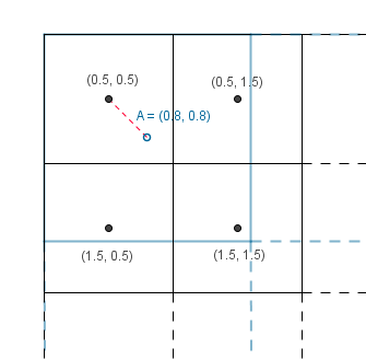
Let us first see upscaling. Assume we have a 4×4 texture and we want to render it to a 5×5 area.

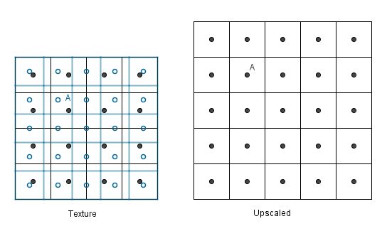
Consider the pixel A. We would need to have a value in the texture located at the mapped A (left image, blue, empty dot). Alas we have no value there, but we have values near it (the black dots).

There are two simple ideas how we could get that value. The simplest is that we could look at the nearest neighbour and take its value.

This is really fast, but usually the result is blocky and not desired. Remember, the image was a discrete sample from an analogue signal. This means that there is a value between the samples and it is most probably not the ones we sampled, but something in between.

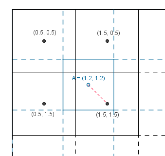
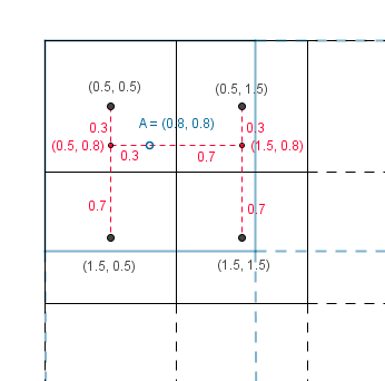
In order to get a value in between in 1D we can look at the closest values and take the weighted average depending on the distance to those values. The unknown value would be a convex combination of the neighbouring values, this is called linear interpolation.

With our 2D texture we could calculate the direct distances to the 4 neighbours and use the same approach. However calculating the distances would include a square root. More faster, but still effective, way would be to use bilinear interpolation. That means that we first interpolate linearly in one direction and then interpolate the results linearly in the other direction.

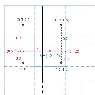
We will get the same result no matter which way we interpolate first. Result has the color values considered by the $(1-distanceX) \cdot (1-distanceY)$ factor if the known values are unit distance apart from each other.

Downscaling

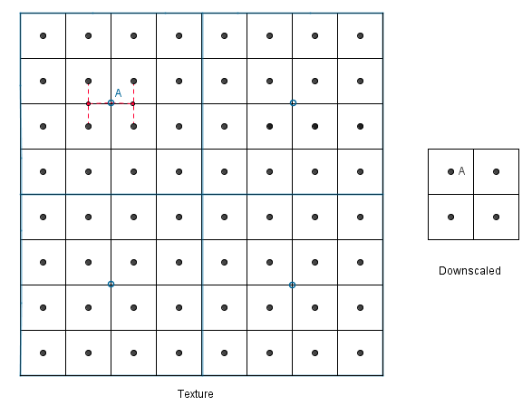
What about the other way around? Let us have a 8×8 texture that we want to render to a 5x5 area. 

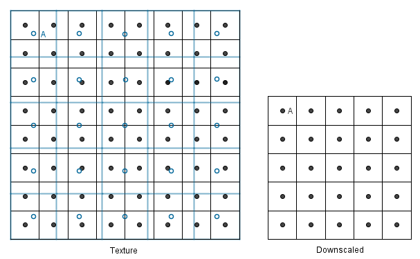
We have again the same two simple approaches. We first map our down downscaled coordinates to the texture, then we can find the nearest neighbour to each of the unknown values (again blue empty circles).

Or we could find the nearest 4 neighbours and do the bilinear filtering again.

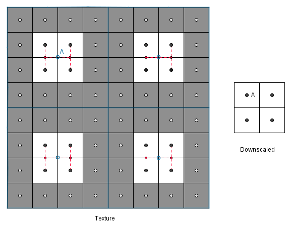
But there is a problem. With upscaling it does not matter how much we upscale, there are always 4 neighbours that we can interpolate. However, with downscaling it might happen that our new value should involve more than 4 neighbours to be correct. This will happen if we want to upscale more than 2 times the known texture size.

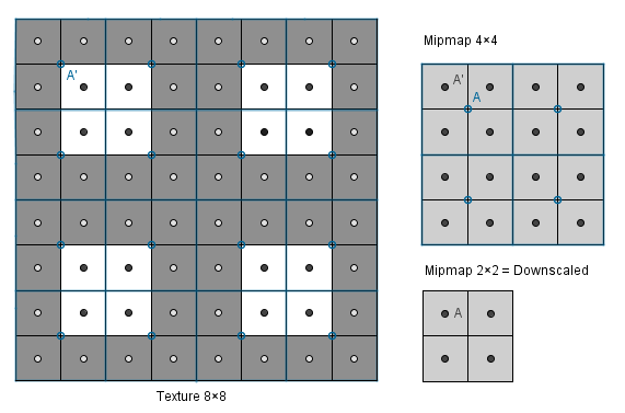
Consider if we would want to render the 8×8 texture to a 2×2 area with bilinear filtering.

We would have to consider all of the 16 values that should be in the mapped pixel, otherwise we will miss out in a lot of data and produce artifacts. Think if the 1th, 4th, 5th and 8th column would consist of black values and everything else is white. With just the bilinear approach we would not see anything that would indicate those black lines in the 2×2 area. Even though exactly half of the original image was black. We could even have some rows black and still the final image would be totally white. This is not desirable and next we will see what can be done about it.

Mipmap

As you saw, there is a significant problem, if we downscale an image more than 2 times with bilinear interpolation. This is why usually there are mipmaps accompanying the texture (our image). Mipmaps are precalculated exactly 2 times smaller versions of the texture. 

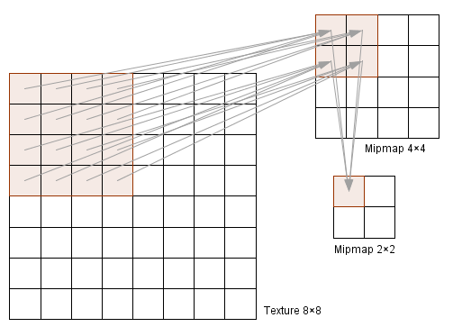
Even though our initial texture was 8×8, we can now use the mipmaps 4×4 to downscale to 3×3 and avoid the problem of missing out on some values. Notice that when generating mipmaps, exactly 2 times smaller mipmap holds for each value the equal weighted average of all 4 neighbouring pixel values from the bigger image. This will of course create some other problems, for example the checkerboard texture will at one point just be a equally gray image.

128×128	64×64	32×32	16×16	8×8	4×4

As you notice the sizes are of a power of two. This is because this way GPU can divide the dimensions more efficiently and the texture always divides by 2 (down to 2×2 or 1×1). This means that the dimensions of the textures should always be a power of two. If they are not, the mipmaps may not be automatically calculated for you. Of course you could always find the mipmaps yourself and send them along with the texture to the GPU.

Now, when we generate the mipmaps, we will solve the problem that the downscaled images are missing values from some pixels.

The values are there, but the number of pixels is too small to represent the pattern, so the smaller mipmaps just have gray values (instead of the black and white pattern).

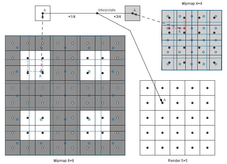
Ok, but what about if we want to render the image with a size somewhere between the mipmaps? Do we use a larger mipmap and downscale or the smaller mipmap and upscale? It would make more sense to use the larger one, because it contains more data we can use. On the other hand, if we are closer to the smaller mipmap, then we should perhaps use that, because the result will resemble that one more (we will just calculate quite a similar result again from the larger one).

This comes back to getting to know unknown values from between known values, thus we can interpolate between the mipmaps. With interpolation we again have two simple choices, just take the nearest neighbour (no meaningful interpolation) or interpolate linearly between them. The last option will be trilinear filtering, if bilinear filtering is applied in both of the mipmaps.

Below is an example when we want to render the image in a 5×5 area and we have mipmaps 4×4 and 8×8. The value 5 is three quarters away from the value 8 and one quarter away from the value 4. So we can go do a bilinear filtering in both of the mipmaps and then do another linear filtering on the results, resulting in a trilinear filter.

This is good, because sequential mipmaps might have quite distinct values in them. So when we are looking at a plane at a grazing angle, then several mipmaps are used for that plane. This means that a smooth transition from one mipmap to another is preferred.

You can check this out in the example on the right. With no mipmaping you can see that the pattern far away is sharp, but does not represent the checkerboard. With bilinear filtering you can notice sharp mipmap transitions happening along the plane. With trilinear filtering the result is much better.

There is another problem, though. The pixels in the distance become all gray, but in reality we should see some pattern there. At least in the horizontal direction. The problem comes from the fact that we are downscaling the mipmaps equally in both directions i.e. isotropically. So if our pixel covers an area, that has significantly more height then width in the texture, then the mipmap is still chosen the minimum that covers the area.

For example if our pixel covers 2×8 area in the texture, we will find a mipmap where 8 textures values are represented as 1 value. This would be the ideal mipmap if our pixel would cover 8×8 area, but currently 75% of the information we get from the mipmap is bogus. We should rather take the mipmap where 2 texture values are covered by one, and then sample 4 times from it and average the results. This kind of sampling is called anisotropic filtering and it will give sharper and more correct results when the texture in the result should not be scaled equally in both directions.

In the previous interactive sample you can change the number of samples taken along the widest direction. Note that with the perspective projection our pixels actually cover a trapeze shaped area in the texture. You can read more about anisotropy here and here.

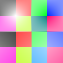
You might also thing about storing the textures for multiple objects in a single image file. This would be called an atlas and mipmapping that might cause texture bleed or texture pollution. For example consider the following atlas:

128×128	64×64	32×32	16×16	8×8	4×4	2×2	2×2 enlarged

Texture bleed does not happen, because our textures are inside the 2-power lines of the texture. Remember how the mipmaps were downscaled, there are lines in the image where the values left of the line and values right of that are mixed only if we have scaled too much. One example of that are the lines in the middle of the image. Those will be crossed if we have downscaled to 1×1 image. Here we have downscaled to 2×2 and you can see that the quarter lines have been crossed and there is texture pollution. In order to avoid that we should specify the minimum scale we want for this atlas.

You can read more about using atlases with mipmaping here.

Finally, here is another example where you can try out different minification, magnification filters and anisotropy levels.

Aliasing

As you might have noticed in the previous examples with the checkerboard pattern there were some weird effects if we tried to map it to a small area. You can try it out by making the cube in the previous example small and not use any mipmapping (min. filter linear or nearest neighbour). You can use mipmapping and even anisotropy also, the effect is still there, although not that clearly visible.

It comes from the fact that our signal in the image has a too high frequency to be displayed correctly with such a small amount of samples. Nyquist-Shannon sampling theorem says that in order to be able to fully construct a periodic signal, we should sample more than two times in a period. Of course more is better, but if we sample less we will definitely not get the original signal back, we will get something else - an alias of it. Aliases are artifacts in the image that are not supposed to be there: we are seeing something that was not originally there. You can read more about the meaning of Nyquist-Shannon sampling theorem here.

Consider a high frequency sine wave with a period of $\pi$ and let us sample it about 1.5 times per period (not >2 like Shannon suggests). This is what we will get:

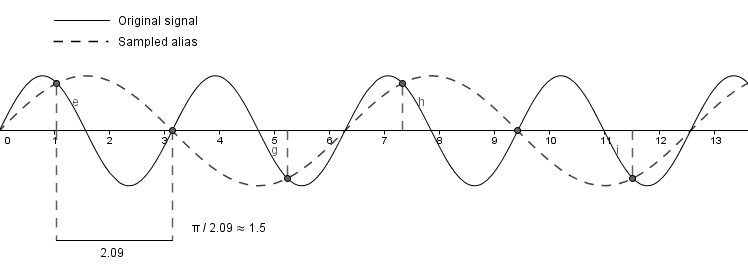
As you can see, based on the samples we will visually see another sine wave that has a smaller frequency. But this sine wave was not there in the original signal. Our samples indicate a function $sin(x)$, but in reality we had $sin(2x)$.

This kind of aliasing produces Moire patterns and it also happened with the checkerboard and cube examples before. In order to see how devastating that effect can be, consider a function $cos(x^2 + y^2)$. As you remember, our textures do not have to be discrete images, but we could have a mathematical function that defines the intensity. So let us take that function. Let us also scale it to be in the range $[0, 1]$, so it will be:

$\dfrac{cos(x^2 + y^2)}{2} + 0.5$.

Below is a graph of a one dimensional function. You can see that the frequency increases as the coordinates increase.

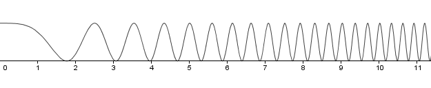
In the example on the right we will render it to 300×200 area (the size of the graphical box of the example). But this is an infinite function, we have to decide how much of we will render. The slider below controls the sample step. For readability it denotes a factor or the coordinates. So if it is 1, we will render 1×1 area to the viewport. If you increase it to 2, it will be a 2×2 area of the aforementioned function. As you can see, increasing it over 10 will start to produce a lot of Moire patterns. This is exactly because we are trying to fit a high frequency signal to our 300×200 area without having enough pixels to represent the signal correctly.