Frames of Reference and Projection
In this chapter we will see different frames of references that one should think about when doing computer graphics. We have already seen previously that there is a notion of a scene graph and sub-objects can have their local transformations that are made together with some parent object transformations. There are a couple of more dependencies among different frames of references when it comes to the actual rendering of our objects.
We will also see how the actual projection of our 3D world is done to a 2D screen. There are few different types of projections one could do and some parameters for them that will affect the final result.
Some definitions that are used in this chapter:
- Frame of reference – a coordinate system in which we are currently representing our objects in.
- Object space – a frame of reference from a specific object.
- World space – a frame of reference from our world coordinate system.
- Camera space – a frame of reference from our camera.
- Clip space – a frame of reference used to define a portion of our world that is actually visible from a camera.
- Screen space – a frame of reference from our screen's coordinate system.
- Clipping – idea of ignoring the vertices or objects that are not visible for our camera.
- Orthogonal matrix – matrix, whose rows and columns are orthogonal unit vectors. Inverse of it equals the transpose of it.
- Cross product – operation between vectors that creates another vector orthogonal to the operands. $u×v = (u_y v_z - u_z v_y, u_z v_x-u_x v_z, u_x v_y - u_y v_x)$.
Frames of Reference
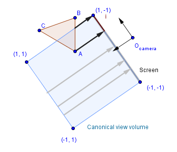
Computers will do exactly what you tell them to do. The question is about understanding what do we actually want to do and explaining that to a computer with enough rigor. For example we might want the computer to render a square, but this sentence is way too abstract for the computer to understand. More rigorous way to think about this is that we want lines between pairs of vertices $(1, 1)$, $(-1, 1)$, $(-1, -1)$ and $(1, -1)$, that are represented in the world space, to be drawn in a 400×300 area of the screen so that there is a linear mapping:
$[-4, 4]×[-3, 3] \rightarrow [0, 400]×[0, 300]$.
This will already specify which pixels to color for our vertices. For example the vertex $(1, 1)$ would be drawn on the pixel located at coordinates $(250, 200)$. Here you might notice a couple of problematic things:
- Our geometry will be mirrored in the y direction, because in our world space y will point up, but in the screen space, y will point down.
- We are mapping from 2D to 2D. How to do it from 3D to 2D? What if we are not looking from the positive z direction?
On the other hand we might notice that with this kind of mapping our scene would always show the same amount of the scene if the resolutions changes. Although we might want to change that also.
There are actually many frames of references and transformations between our vertices and what we see on the screen. Let us look at them one at a time.
World Space
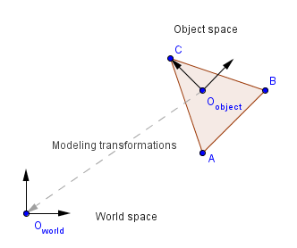
First, our vertices are usually defined in the object space. We will try to center our object around some object origin ($O_{object}$) that will serve as the scaling and rotation fixed point. Our object is located somewhere in the world space though, so we will use modelling transformations to represent the vertices with world space coordinates. Imagine if there are multiple triangles, they can not all be located in the world space origin, they are probably scattered all around the world space, and thus each have distinct world space coordinates. Although they might have the same object space (local) coordinates.
Camera Space
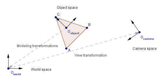
Secondly, there is a camera somewhere in the world space. This camera has its own coordinates in the world space and is transformed just like any other object / vertex. Our goal here is to position everything into camera space so that camera and world frames match. In other words, transform everything so that camera will be located at the world origin and the axes will be aligned.
Usually there is a function called lookAt(), where you can say where in the world is your camera located, which is the up direction and to what point is it pointed (is looking) at. This is a convenience function that underneath will construct the corresponding matrix that will do the camera transformation in this step. Let us see, how this can be done.
We know:
- Camera's position in world space. Call it $p$.
- Camera's up-vector. Call it $u$.
- Camera's looking direction. Call it $l$.
Well, the first step would be to align the origins. So we want to move all our objects so that the camera would be in the world origin. We had a translation $p$ that moved camera away from the origin, so the reverse would be just $-p$.
So the first transformations would be:
$\left( \begin{array}{cc}
1 & 0 & 0 & -p_x \\
0 & 1 & 0 & -p_y \\
0 & 0 & 1 & -p_z \\
0 & 0 & 0 & 1
\end{array} \right)$
Next we need to align the axes. Now, the vector $l$ shows the direction we are facing, but because the z-axis should be in the negative direction, we will reverse it: $w = -l$. We assume that vectors $u$ and $w$ are orthogonal to each other and of unit length. We still need one orthogonal vector, the right vector, in order to have the camera basis. We could use the Gram-Schmidt process here, but a more simpler way to find an orthogonal unit vector, given already two, would be to use the cross product of vectors. So $v = w×u$. Notice that the cross product is not commutative and will follow the right-hand rule. The vector $v$ will emerge from the plane defined by $w$ and $u$ in the direction where the angle from $w$ to $u$ will be counter-clockwise. If you exchange $w$ and $u$ in the cross product, then the result will point to the opposite direction.
Now we have the vectors $u$, $v$ and $w$ that are the basis of the camera's frame of reference. The transformation that would transform the camera basis from the world basis (ignoring the translation for now) would be:
$\left( \begin{array}{cc}
u_x & v_x & w_x & 0 \\
u_y & v_y & w_y & 0 \\
u_z & v_z & w_z & 0 \\
0 & 0 & 0 & 1
\end{array} \right)$
Remember that we can look at the columns of the matrix to determine how the basis would transform. But that would be the transformation which would transform the camera space (coordinates) to the world space. We need to find a transformation to get from world space to camera space. Or in other words, transform the camera basis to be the current world space basis. You might remember from algebra that the inverse of an orthogonal matrix is the transpose of it. All rotation matrices are orthogonal matrices and a multiplication of two rotation matrices is a rotation matrix. Our camera basis will differ from the world basis only by a number of rotations. So in order to find out how to transform the world so that the camera basis would be aligned with the world basis, we only need to take the inverse of those rotation. That is the inverse of the matrix we just found. The inverse is currently just the transpose of it.
The total view transformation would be then:
$V = \left( \begin{array}{cc}
u_x & u_y & u_z & 0 \\
v_x & v_y & v_z & 0 \\
w_x & w_y & w_z & 0 \\
0 & 0 & 0 & 1
\end{array} \right)
\left( \begin{array}{cc}
1 & 0 & 0 & -p_x \\
0 & 1 & 0 & -p_y \\
0 & 0 & 1 & -p_z \\
0 & 0 & 0 & 1
\end{array} \right)$
In some sources the view transformation is called the inverse of the camera transformation. There the camera transformation is the transformation that transforms the actual camera as an object. In other sources the camera transformation is the transformation that transforms all the vertices into the camera space. One should explain what is actually meant when using those terms. The term view transformation (the view matrix) is generally more common.
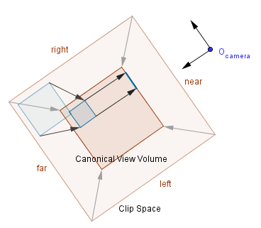
Clip Space
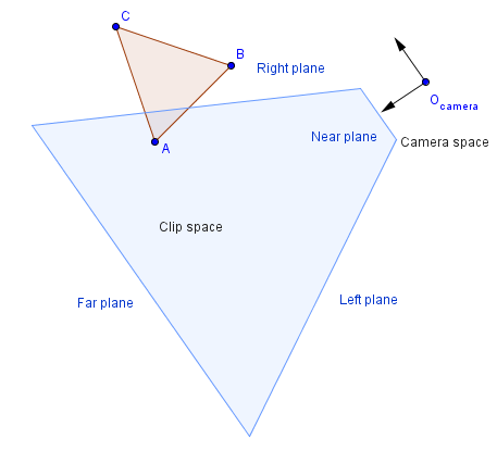
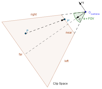
Third step is to construct the clip space. This is the space that should be seen from the camera. In our illustration here there is a 2D projection of it. In 3D you will also have a top and a bottom plane. Based on the transformation you might have to specify those plains directly or, as is the case with perspective projection, you can specify a field of view parameter that will calculate those itself.
Everything outside this clip space is clipped, i.e. ignored in rendering. It might depend on what kind of clipping techniques are in use. For example if a line crosses the clip space, then it might be segmented: another vertex is created at the border of the clip space. Objects that are wholly outside of the clip space, are ignored. This is one place where we want to be able to determine the rough locations of our objects quickly. Later we will see different methods (e.g. binary space partitioning, bounding volume hierarchy) that help to determine that. Mathematically you can think that the equations of the planes are constructed and intersections with other planes (ones defined by all of the triangles in the scene) are checked for. Of course, if we are only interested about vertices, then we can put every vertex in the plane equation and see which side of the plane a vertex lies.
We will look this and the next step in more detail when talking about different projections.
Canonical View Volume
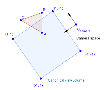
Fourth step is to transform everything so that the clip space will form a canonical view volume. This canonical view volume is a cube in the coordinates $[-1, 1]×[-1, 1]×[-1, 1]$. As you can see from the previous illustration we had kind of a weird shape for the clip space. This shape is a frustum of a pyramid in the case of perspective projection. In computer graphics we call it the view frustum. Transforming that into a cube will transform the whole space in a very affecting way. This is the part where we leave the world of affine transformations and perform a perspective projection transformation. It is actually quite simple, we will just put a non-zero value in the third column of the last row of our transformation matrix. As you remember, affine transformations needed the last row to be $(0, 0, 0, 1)$, but for perspective transformation we will have $(0, 0, p, 0)$. Depending on how an API is implemented, we might have $p=1$ or $p=-1$ or even something else. After this transformation, there is a need for the perspective division, because the value of w will usually no longer be 1. Remember that in homogeneous coordinates $(x, y, z, w) = (x/w, y/w, z/w)$.
As you can see, coordinates will be divided based on the value of w, which will depend on the value of z. This actually causes the objects further away to be projected smaller then objects that are closer to the camera - the same way we see the world.
Screen Space
Final step is to project the canonical view volume into screen space. Our screen has usually mapped the coordinates of pixels so that $(0, 0)$ is in the top-left corner and positive directions are to the right and down. Depending on the actually screen resolution (or window / viewport size if we are not rendering full-screen), we will have to map the canonical view volume coordinates to different ranges. In either way, this will just be a linear mapping from the ranges $[-1, 1]×[-1, 1] \rightarrow [0, width]×[0, height]$ like we saw in the beginning.
This mapping is called the viewport transformation and the matrix that does it is quite simple. This step is usually done automatically. For the proportional linear mapping from one range into another we just need to scale the initial range to be of the same length as the final range, and then translate it so that they cover each other.
The length of the range $[-1, 1]$ is 2. For the length of the range $[0, width]$ we will take width. This is because we want the value -1 mapped to 0 and the value 1 mapped to width. So the scaling should be by $\frac{width}{2}$, after which we will have a range $[-\frac{width}{2}, \frac{width}{2}]$. Then we will just translate by $\frac{width}{2}$ and end up with a range $[0, width]$.
$
\left( \begin{array}{cc}
x_{screen} \\
y_{screen} \\
z_{canonical} \\
1
\end{array} \right) =
\left( \begin{array}{cc}
\frac{width}{2} & 0 & 0 & \frac{width}{2} \\
0 & \frac{height}{2} & 0 & \frac{height}{2} \\
0 & 0 & 1 & 0 \\
0 & 0 & 0 & 1
\end{array} \right)
\left( \begin{array}{cc}
x_{canonical} \\
y_{canonical} \\
z_{canonical} \\
1
\end{array} \right)
$
Notice that the z value is brought along here. This is useful in order to later determine which objects are in front of other objects. Also the y values still seem to be reversed. This will be handled later by OpenGL, currently we just assume that the $(0, 0)$ in the screen space is at the bottom-left corner and the positive directions are up and right. Also the z value will later be normalized to a range $[0, 1]$.
Projections
We just saw a number of steps that occur, when we want to transform our 3D space to a 2D screen. Basically there are three things that need to happen:
- View transformation (represent our coordinates in the camera basis).
- Convert a clip space into the canonical view volume.
- Project the canonical view volume to the screen or viewport of specific dimensions i.e. the viewport transformation.
There is actually an intermediary step between 2. and 3. – the perspective division. This will convert our homogeneous coordinates back to points. Coordinates in a form $(x, y, z)$, where $x = \frac{x_{hom}}{w}$, $y = \frac{y_{hom}}{w}$, and $z = \frac{z_{hom}}{w}$ are called normalized device coordinates at this stage. The perspective division, as the name suggests, is essential for the perspective projection.
As you see, the view transformation is only dependent on the camera. The viewport transformation depends on the size of our viewport (e.g. screen). The place, where we determine what kind of projection we are actually performing, is defining the clip space. Note that from the computer's point of view there is again a matrix that performs the described conversion: converts a frustum, parallelepiped, cuboid into a cube $[-1, 1]^3$.
There are three main projections that are more often used: the orthographic, oblique and perspective projections.
Orthographic Projection
This is the simplest one that uses another cube as the clip space. This cube is defined by 6 planes: $x = left$, $x = right$, $y = bottom$, $y = top$, $z = near$, $z = far$. The only thing a projection matrix needs to do, is to transform that area into the clip space. Now, there is actually no requirement that the planes are somehow symmetric, e.g. $left = -right$. It might not be so, and thus the projection matrix must take that into account.
Let us see how to transform the x coordinate into the canonical view volume. We have $x \in [left, right]$. First we want to scale that range to be of length 2. So our matrix will perform the scaling first. We scale by a value that first creates a range of unit length (divides by the length of the previous range) and then multiplies that by 2.
$ \left( \begin{array}{cc}
\frac{2}{right - left} & 0 & 0 & \_ \\
\_ & \_ & \_ & \_ \\
\_ & \_ & \_ & \_ \\
0 & 0 & 0 & 1
\end{array} \right)
$
Notice that this is the same thing that we also need to do with y and z coordinates. With the latter the $near$ actually has a bigger value than $far$, because the z axis is inverted.
$ \left( \begin{array}{cc}
\frac{2}{right - left} & 0 & 0 & \_ \\
0 & \frac{2}{top - bottom} & 0 & \_ \\
0 & 0 & \frac{2}{near - far} & \_ \\
0 & 0 & 0 & 1
\end{array} \right)
$
Now we have scaled everything to be of correct length, but we might be positioned wrongly. Next we need to translate it so that the midpoint would be mapped to 0 in our scaled system. The midpoint of the range $[left, right]$ would be $\frac{left + right}{2}$. Because we have already scaled our world, then we also need to scale this midpoint first. So we will multiply it with our scale factor:
$\frac{left + right}{2} \cdot \frac{2}{right - left} = \frac{right + left}{right - left}$.
This is the distance we need to translate (in the opposite direction) for the midpoint of the current space to be at 0 of the target space. Because our range is of length 2, then $left \rightarrow -1$ and $right \rightarrow 1$.
$ \left( \begin{array}{cc}
\frac{2}{right - left} & 0 & 0 & -\frac{right + left}{right - left} \\
0 & \frac{2}{top - bottom} & 0 & -\frac{top + bottom}{top - bottom} \\
0 & 0 & \frac{2}{near - far} & \frac{near + far}{near - far} \\
0 & 0 & 0 & 1
\end{array} \right)
$
This is the same result you would come to if you would first translate the midpoint and then scale. In that case you would have to multiply the matrices together and the resulting matrix is the same we just derived.
Depending on how one chooses the clip planes, orthographic projection transforms a cube or a parallelogram into a cube. Objects further away from the camera are of the same size as those closer. As you can see from the example below, a projected cube has both the face near the camera and the one in the back projected to the same coordinates.
Sometimes one might also want to add a zoom capability to this projection. If the planes are symmetric, then the zoom can just be a factor which divides the plane values. This will make the clipping box be smaller and thus the projected objects larger.
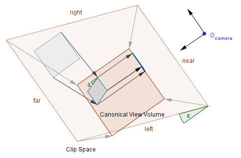
Oblique Projection
This is quite similar to orthographic projection, but a shear-xy is applied to the space before. The clip space is thus a parallelepiped. For the shear-xy transformation we can have values $\alpha_x$ and $\alpha_y$ for the x and y axis tilt angle. Sometimes a cotangent of those angles is used. It does not really matter, because $cot(\alpha) = tan(\frac{\pi}{2} - \alpha)$, so just the direction of the shear would be different.
Although we could shear by an arbitrary amount, there are two $\alpha$ values that have the most use:
- Cavalier projection – One angle is fixed at $\alpha_y = 45°$. Another angle is free, but lines perpendicular to the z plane must preserve their length.
- Cabinet projection – One angle is fixed at $\alpha_y \approx 64.3°$. Another angle is free, but lines perpendicular to the z plane must be half their length.
In order to satisfy the conditions for the lengths of the perpendicular line segments, we can use the sine and cosine functions for the shear value calculations. So instead of:
$ \left( \begin{array}{cc}
1 & 0 & tan(\alpha_x) & 0 \\
0 & 1 & tan(\alpha_y) & 0 \\
0 & 0 & 1 & 0 \\
0 & 0 & 0 & 1
\end{array} \right)
$
We would have for cavalier projection:
$ \left( \begin{array}{cc}
1 & 0 & cos(\alpha_x) & 0 \\
0 & 1 & sin(\alpha_x) & 0 \\
0 & 0 & 1 & 0 \\
0 & 0 & 0 & 1
\end{array} \right)
$
Or for the cabinet projection:
$ \left( \begin{array}{cc}
1 & 0 & \frac{cos(\alpha_x)}{2} & 0 \\
0 & 1 & \frac{sin(\alpha_x)}{2} & 0 \\
0 & 0 & 1 & 0 \\
0 & 0 & 0 & 1
\end{array} \right)
$
When you multiply those shear-xy matrices with an orthographic projection matrix, then you get an oblique projection matrix. Those kinds of projections are used in engineering or magazines, but also in different games.
Perspective Projection
This is probably the most common projection, because it emulates the way we see the world around us. When we are talking about 3D graphics, we usually want to create an immersive illusion that resembles our own look on the world around us. As mentioned, this is also the place where homogeneous coordinates give us a simple way to achieve the desired projection. We want the final coordinates to be all directly dependent on the z coordinate. With ordinary affine transformations they are not, we can add a multiple of the z coordinate to the values, but we can not have the whole coordinate to be a factor of the z value. With homogeneous coordinates all coordinates are a factor of the w value that has until now been 1 for points.
The homogeneous point $(x, y, z, w)$ is actually a point $(x/w, y/w, z/w)$.
Because of that we have to leave the world of affine transformations and change the bottom row of our projection matrix. We can assign the negative z value to the w value. This will also invert the z axis. In OpenGL the positive z axis in the clip space will point in the opposite direction as the z axis in the camera space. That is also why the scale factor for the z coordinate has been a negative value in the previous matrices.
We here again have the near, far, left, right, top and bottom values. The near and far values are the corresponding planes, but the left, right, top and bottom values are the boundaries of the near plane. Those values will define the whole frustum that has a peak in the camera's position. We could think of this projection as transforming the frustum into a cube like before.
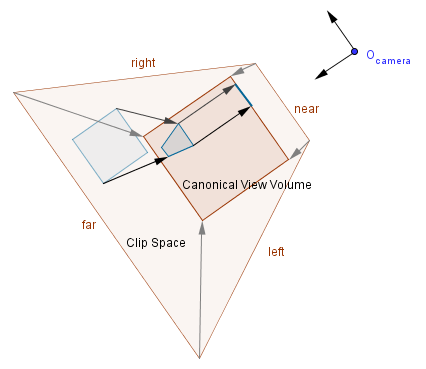
Usually however it is more convenient to define a field of view, rather than specifying the left, right, top and bottom values. Field of view is the angle $\alpha$ that specifies the vertical viewing angle. There is also a value called aspect ratio that is the ratio between the viewport's horizontal and vertical lengths. In order to further simplify things, we can define the projection plane to be the near plane. Notice that before the near plane and the projection plane have been different. We can also say that the projection plane has the height of 2 and the width of 2 times the aspect ratio.
Now, we have an arbitrary point $P$ in our frustum and a projection of that point $P'$ in the near plane.
We want to know that is the new y coordinate of our point. We can use similar triangles to find that out. Notice that our points have to lie on the same line that also passes the camera. Also both points have some distance from the FOV angle bisector. That bisector is the $y=0$, $x=0$ line, ie the z axis.
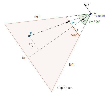
Because of the similar triangles we have $\dfrac{P_y}{P'_y} = \dfrac{P_z}{P'_z} \rightarrow P'_y = \dfrac{P_y \cdot P'_z}{P_z}$. As we agreed on the height of the projection plane, we can calculate the value of $P'_z$ from trigonometry: $tan(\frac{\alpha}{2}) = \dfrac{1}{P'_z}$. So $P'_z = \dfrac{1}{tan(\frac{\alpha}{2})}$. This means that:
$P'_y = \dfrac{P_y}{P_z \cdot tan(\frac{\alpha}{2})}$.
The division by the z coordinate is done later, but we can put the scale factor directly into the matrix now. For the x coordinate we need to look at the horizontal angle, which we do not know. We know that the tangent of that unknown $\frac{\beta}{2}$ would be used the same way as it was with $\frac{\alpha}{2}$. The tangent of that would be $\frac{aspectRatio}{P'_z}$. We can get that value by multiplying the calculation of the vertical angle tangent by the value of aspectRatio.
$tan(\frac{\alpha}{2}) = \dfrac{1}{P'_z}$
$aspectRatio \cdot tan(\frac{\alpha}{2}) = \dfrac{aspectRatio}{P'_z}$
This will be the scale factor for the x coordinate.
$ \left( \begin{array}{cc}
\dfrac{1}{aspectRatio \cdot tan(\frac{\alpha}{2})} & 0 & 0 & 0 \\
0 & \dfrac{1}{tan(\frac{\alpha}{2})} & 0 & 0 \\
0 & 0 & \_ & \_ \\
0 & 0 & -1 & 0
\end{array} \right)
$
There is still one thing missing. We want to bring the z value along as is, but because w is no longer 1, we can not just use the same formula we did with orthographic and oblique projections.
Previously we had $scaleZ \cdot z + translateZ$. This result is however divided by $-z$ (because $w$ has the value of $-z$) later on. So we have to find another $scaleZ$ and $translateZ$ for the equation:
$-scaleZ - \frac{translateZ}{z}$.
Now, we know two values for this equation, the endpoints in the near and far planes should be mapped to -1 and 1 respectively. Note that the $near$ and $far$ values are usually given as positive values in graphics libraries. As our $z$ axis in view space is pointing to behind the camera, we need to negate the $near$ and $far$ values. So the following derivation and matrix will hold, when you use the positive parameter values to represent the negative coordinates.
$-scaleZ - \frac{translateZ}{-near} = -1$
$-scaleZ - \frac{translateZ}{-far} = 1$
We can get rid of the minuses:
$-scaleZ + \frac{translateZ}{near} = -1$
$-scaleZ + \frac{translateZ}{far} = 1$
When we bring the $translateZ$ value to one side of the equation:
$translateZ = near \cdot (scaleZ - 1)$
$translateZ = far \cdot (scaleZ + 1)$
This means that:
$near \cdot (scaleZ - 1) = far \cdot (scaleZ + 1)$
$near \cdot scaleZ - near = far \cdot scaleZ + far$
$- near - far = far \cdot scaleZ - near \cdot scaleZ$
$- (near + far) = scaleZ \cdot (far - near)$
$scaleZ = \frac{near + far}{near - far}$
We can substitute that back to find the translation's value.
$-\frac{near + far}{near - far} + \frac{translationZ}{near} = -1$
$-\frac{near + far}{near - far} + 1 = -\frac{translationZ}{near}$
$-\frac{near + far}{near - far} + \frac{near - far}{near - far} = -\frac{translationZ}{near}$
$\frac{- near - far + near - far}{near - far} = -\frac{translationZ}{near}$
$\frac{- 2 \cdot far }{near - far} = -\frac{translationZ}{near}$
$-near \cdot \frac{- 2 \cdot far }{near - far} = translationZ$
$translationZ = \frac{2 \cdot far \cdot near }{near - far}$
So our final matrix would be:
$ \left( \begin{array}{cc}
\dfrac{1}{aspectRatio \cdot tan(\frac{\alpha}{2})} & 0 & 0 & 0 \\
0 & \dfrac{1}{tan(\frac{\alpha}{2})} & 0 & 0 \\
0 & 0 & \frac{near + far}{near - far} & \frac{2 \cdot far \cdot near }{near - far} \\
0 & 0 & -1 & 0
\end{array} \right)
$
Now, this does map to the correct range for z values, but the mapping is not a linear one. Previously we had a linear mapping, but with perspective projection a linear mapping is not possible. The best we can do is have it map to the correct range and keep the order between points.
Imagine that our near plane is at 1 and far plane is at 10. This is how the z values would be mapped:
| 1 | 2 | 3 | 4 | 5 | 6 | 7 | 8 | 9 | 10 | |
|---|---|---|---|---|---|---|---|---|---|---|
| Linear | -1 | -0.77 | -0.55 | -0.33 | -0.11 | 0.11 | 0.33 | 0.55 | 0.77 | 1 |
| Perspective | -1 | 0.11 | 0.48 | 0.66 | 0.77 | 0.85 | 0.90 | 0.94 | 0.97 | 1 |
As you can see, the values that are more closer to the far plane, are mapped more closer together than those near the near plane. Because of that there might be more errors in determining the order of objects further away. This might cause z-fighting for those faraway objects.