Parametric Curve Construction

You are probably aware of an implicit way to represent a function. We can also represent curves implicitly to specify an algebraic relation between the coordinates.

For example consider a cubic function:

$f(x) = b_0 + b_1 \cdot x + b_2 \cdot x^2 + b_3 \cdot x^3 = y$

This will define a relationship between $x$ and $y$. We could use it to put in values for $x$ and get out the values for $y$. Or we could put in both the $x$ and $y$, and see if the equation holds. This would test if a given point is on the curve or not.

What we would want, however, is that we have some other parameter $t$ that we input, and we get out the points $(x, y)$ that are on our curve. It would be even better, if we would know that for a given $t$, where roughly the points will come out. So if we are interested in a certain area of the curve, we can get out the points inside that area. That would be a function:

$g(t) = a_0 + a_1 \cdot t + a_2 \cdot t^2 + a_3 \cdot t^3$

where $a_i \in R^2$ or $a_i \in R^3$ depending if we are in 2D or 3D. Respectively it would give out points in the corresponding dimension. You can notice that depending on the dimensionality we can just think of that many equations in 1D. It is more concise to rather think about vector equations, where the coefficients are from a vector space. I.e. a curve in 2D or 3D is just 2 or 3 curves in 1D for each of the coordinates.

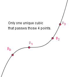
As you know, a cubic curve can be uniquely defined by giving 4 points. It would seem in our best interest to somehow specify those 4 points and have the curve pass through them. We can do this, because a cubic equation has 4 unknowns (our $a_i$). If we specify 4 constraints, we can find those currently unknown coefficients and thus make $g(t)$ actually usable.

If we want a cubic curve to pass through all 4 points (called control points), we can specify the constraints:

$g(0) =  a_0 + a_1 \cdot 0 + a_2 \cdot 0 + a_3 \cdot 0 = p_0$

$g(\frac{1}{3}) =  a_0 + a_1 \cdot \frac{1}{3} + a_2 \cdot \left (\frac{1}{3} \right)^2 + a_3 \cdot \left (\frac{1}{3} \right)^3 = p_1$

$g(\frac{2}{3}) =  a_0 + a_1 \cdot \frac{2}{3} + a_2 \cdot \left (\frac{2}{3} \right )^2 + a_3 \cdot \left (\frac{2}{3} \right)^3 = p_2$

$g(1) =  a_0 + a_1 \cdot 1 + a_2 \cdot 1 + a_3 \cdot 1 = p_3$

The control points $p_i$ are called parameters, so a vector $\textbf{p}$ would be a parameter vector.

We can write this system of equations as a matrix-vector operation.

$\textbf{C} \cdot \textbf{a} = \textbf{p}$

We call the matrix $\textbf{C}$ a constraint matrix.

$\textbf{C} =  \left( \begin{array}{cc}
1 & 0 & 0 & 0 \\
1 & \dfrac{1}{3} & \left (\dfrac{1}{3} \right )^2 & \left (\dfrac{1}{3} \right )^3 \\
1 & \dfrac{2}{3} & \left (\dfrac{2}{3} \right )^2 & \left (\dfrac{2}{3} \right )^3 \\
1 & 1 & 1 & 1
\end{array} \right)
$

There is also the coefficient vector $\textbf{a}$. Those are currently the unknowns – the coefficients of a particular parametric polynomial equation that satisfies our set constraints.

$\textbf{a} = \left( \begin{array}{cc}
a_0 \\
a_1 \\
a_2 \\
a_3 \\
\end{array} \right) $

And finally a parameter vector $\textbf{p}$.

$\textbf{p} = \left( \begin{array}{cc}
p_0 \\
p_1 \\
p_2 \\
p_3 \\
\end{array} \right) $

Given this system we can find the solution to $a$ by taking the inverse of $C$ and multiplying from the left.

$\textbf{C} \cdot \textbf{a} = \textbf{p}$

$\textbf{C}^{-1} \cdot \textbf{C} \cdot \textbf{a} = \textbf{C}^{-1} \cdot \textbf{p}$

$\textbf{a} = \textbf{C}^{-1} \cdot \textbf{p}$

The matrix $\textbf{C}^{-1}$ is called a basis matrix and is usually denoted $\textbf{B}$. This would give us the coefficients that satisfy the equations. We can multiply this equation once more with another vector to get the actual curve equation that we can use. The elements of our new vector $\textbf{t}$ depend on our argument value $t$.

$\textbf{t} = \left( \begin{array}{cc}
1 &
t &
t^2 &
t^3 
\end{array} \right) $

$\textbf{t} \cdot \textbf{a} = \textbf{t} \cdot \textbf{B} \cdot \textbf{p}$

Notice that $\textbf{t} \cdot \textbf{a}$ is exactly our initial curve function $g(t)$. 

$g(t) = \textbf{t} \cdot \textbf{a} = \textbf{t} \cdot \textbf{B} \cdot \textbf{p}$

The product $\textbf{t} \cdot \textbf{B}$ gives us another vector $\textbf{b}$ that has scalar functions as elements. When we multiply it with the parameter vector $\textbf{p}$ we will get a sum of the products of corresponding elements of $\textbf{b}$ and $\textbf{p}$. So each element of $\textbf{p}$ is taken into account, or blended, by a scalar coefficient from $\textbf{b}$. That is why the elements of $\textbf{b}$ are usually called blending functions. They are functions because they depend on our argument $t$. Sometimes our curve function is thus written out as:

$$g(t) = \sum_{i=0}^n b_i(t) \cdot p_i$$

where $b_i(t)$ is the $i$-th element of $\textbf{b}$, a function of $t$.

And now, we have a cubic curve that interpolates 4 control points. We can just sample $t \in [0, 1]$ to get the part of the curve starting from the first control point and ending in the last one. Note that if we were to add more constraints, then the system would become overdetermined for a cubic polynomial, and we could not find a solution. Similarly, we can not have fewer constraints.

So this is the basic idea of constructing a single curve:

1. Pick the parameters and constraints for them,
2. Construct the corresponding constraint matrix,
3. Find the inverse of the constraint matrix – the basis matrix,
4. Construct the blending functions for the parameters,
5. Sample the result.

The cubic curve that we just constructed can be seen in the example on the right. The red values are the control points, you can drag and move them around. The time step is the step we use for sampling the curve. Currently, the curve is just a series of points that have been sampled from our function. In practice, you can do that and connect those points with lines. Or, in newer OpenGL/GLSL versions, there are programmable tesselation shaders. The idea for those is that you can just send to the GPU the control points and those shaders will create the vertices there. Instead of creating the vertices in the application and sending them to the GPU. Sending the data is usually much more expensive than calculating the data on the spot.

But usually, we do not want a curve that is specified with just 4 points. We would want more variation and a longer curve. You can see that if we append another cubic curve to this one (by changing the segment count to 2), then there is a sharp turn where the two curves meet.

A curve that consists of many fixed-degree curves is called a spline. Currently, we would have a spline where each element is an interpolating cubic curve with 4 control points.

When considering curves, we usually want some degree of smoothness. There are two types of smoothness or continuity: parametric $\text{C}$ and geometric $\text{G}$. It is said that a curve has $\text{C}^{~n}$ continuity if it has a continuous n-th derivative everywhere and is also $\text{C}^{~(n-1)}$ for any $n\geq1$. You can see that our cubic spline has $\text{C}^{~0}$ continuity, i.e. where one ends, the other begins. But it does not have $\text{C}^{~1}$ continuity. The derivatives at the end of the first segment and at the beginning of the second segment do not match – there is a sharp corner. Geometric continuity is a bit less restrictive: it needs the derivatives around all curve points to have the same direction, but they could differ in magnitude. The spline we just created, unfortunately does not have that either.

Hermite and Cardinal Curves

As you saw, with 4 points and an interpolating cubic, we got a curve where changing one control point affected the entire curve. If we take higher-order polynomials, then the curve will be affected more, and although we would have a curve that interpolates the points, it is hard to control. Another problem was that if we wanted to make a spline, then just connecting the endpoints would not result in higher smoothness than $\text{C}^{~0}$.

For a spline to be $\text{C}^{~1}$ smooth, we would want derivatives to be the same where one segment ends and another begins. I.e. the derivative must be continuous in the knots.

We specified the constraints so that a curve must pass all of the 4 parameters. All of the parameters were points that the curve interpolated. This does not have to be the case, though. We can have constraints also on the derivatives. Remember, the derivative of a cubic is:

$g'(t) = (a_0 + a_1 \cdot t + a_2 \cdot t^2 + a_3 \cdot t^3)' =  a_1 + 2 \cdot a_2 \cdot t + 3 \cdot a_3 \cdot t^2$

Now, instead of specifying the parameters as points on the curve, we can specify two of the parameters as derivatives on the curve. We will look at the start and end points of the curve.

$g(0) =  a_0 + a_1 \cdot 0 + a_2 \cdot 0 + a_3 \cdot 0 = p_0$

$g'(0) =  a_1 + 2 \cdot a_2 \cdot 0 + 3 \cdot a_3 \cdot 0 = p_1$

$g(1) =  a_0 + a_1 \cdot 1 + a_2 \cdot 1 + a_3 \cdot 1 = p_2$

$g'(1) =  a_1 + 2 \cdot a_2 \cdot 1 + 3 \cdot a_3 \cdot 1 = p_3$

With this system, we can again construct a constraint matrix:

$\textbf{C} =  \left( \begin{array}{cc}
1 & 0 & 0 & 0 \\
0 & 1 & 0 & 0 \\
1 & 1 & 1 & 1 \\
0 & 1 & 2 & 3
\end{array} \right) 
$

to represent the system as a matrix-vector product $\textbf{C} \cdot \textbf{a} = \textbf{p}$.

Finding the inverse $\textbf{B} = \textbf{C}^{-1}$ and multiplying it with our $\textbf{t} = \left( \begin{array}{cc} 1 & t & t^2 & t^3 \end{array} \right)$ will give us corresponding blending functions that when used on the parameter vector will give us our curve. Just like we did before.

This kind of curve is called a Hermite curve. You can see the example on the right. The curve interpolates the control points, and besides those points, you can also change the derivatives at the beginning and end of a curve. When you increase the segment count to get a spline, the next segment has a beginning point the same as the previous segment's end point and the beginning derivative as the previous segment's end derivative.

However, manually controlling the derivatives of a Hermite curve might be tedious. There is a way to calculate the derivatives automatically. For this, we will have to make a curve such that it would interpolate only the second and third points. The first and fourth points will be used to calculate the derivatives by taking a finite difference from the third and second points, respectively.

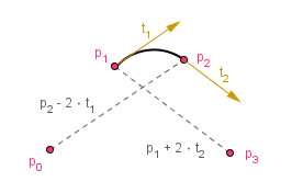
Imagine four control points. The derivative in the second point is half of the vector from the first point to the third point. This will be our constraint. We will parametrize the curve so that at time 0 we are at the second point and at time 1 we are in the third point.

$g(0) = a_0 + a_1 \cdot 0 + a_2 \cdot 0 + a_3 \cdot 0 = p_1$

$g(1) = a_0 + a_1 \cdot 1 + a_2 \cdot 1 + a_3 \cdot 1 = p_2$

If we specify the derivatives so using finite difference:

$g'(0) = 0.5 \cdot (p_2 - p_0)$

$g'(1) = 0.5 \cdot (p_3 - p_1)$

We can add two more constraints that specify our two other parameters $p_0$ and $p_3$:

$p_0 = g(1) - 2 \cdot g'(0) = a_0 - 1 \cdot a_1 \cdot 1 + a_2 \cdot 1 + a_3 \cdot 1$

$p_3 = g(0) + 2 \cdot g'(1) = a_0 + 2 \cdot a_1 \cdot 1 + 4 \cdot a_2 \cdot 1 + 6 \cdot a_3 \cdot 1$

This has given us 4 necessary and sufficient constraints from which we can construct a constraint matrix.

$\textbf{C} =  \left( \begin{array}{cc}
1 & -1 & 1 & 1 \\
1 & 0 & 0 & 0 \\
1 & 1 & 1 & 1 \\
1 & 2 & 4 & 6
\end{array} \right) 
$

This is the constraint matrix for a Catmull-Rom curve. For a spline we can connect individual curves together so that the next segment's first three points are the previous segment's last three points. This will ensure that the first derivatives in the knots are continuous (because they are calculated from the same points).

Sometimes there is an argument called $tension \in [0, 1]$ added. This will change the weight that the derivatives are calculated in the finite difference scheme. Then the derivatives would be:

$g'(0) = 0.5 \cdot (1 - tension) \cdot (p_2 - p_0)$

$g'(1) = 0.5 \cdot (1 - tension) \cdot (p_3 - p_1)$

Notice that when $tension = 0$, then we have the Catmull-Rom curve. When $tension = 1$, then the derivatives are 0, and we have a piecewise linear curve (which does not look like a curve at all). Generally, this curve with varying tension is called a Cardinal curve. It would have another constraint and basis matrices that will depend on the value of $tension$. Some authors call the curves with the $tension$ parameter also Catmull-Rom curves.

You can see this curve in the example on the right. This curve is $\text{C}^{~1}$ smooth and interpolates all the points except the first and the last. Also, changing the locations of points will not affect the whole curve, but only the segments two hops to each direction.

Bezier Curve

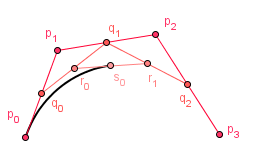
A very important curve in computer graphics is a Bezier curve. We could construct it with a constraint and basis matrices like we did before, but let us try a different approach first. Consider 4 control points $p_0$, $p_1$, $p_2$ and $p_3$ like before. Now, take a linear interpolations between every two consecutive control points with our parameter $t$. We will get 3 points, let us call them $q_0$, $q_1$ and $q_2$. We do the same with those points and find two linear combinations $r_0$ and $r_1$. One more step to go and we get a point $s_0$. 

If you consider a pencil to bet at $s_0$ and interpolate our $t \in [0, 1]$ you will get a curve. Actually you will get a cubic polynomial curve that passes the points $p_0$ and $p_3$, and the derivatives at those points are $3 \cdot (p_1 - p_0)$ and $3 \cdot (p_3 - p_2)$ respectively. In order to see that, let us find out what does our construction actually generate.

We were doing linear interpolation for our points $q_i$:

$q_0 = (1-t) \cdot p_0 + t \cdot p_1$

$q_1 = (1-t) \cdot p_1 + t \cdot p_2$

$q_2 = (1-t) \cdot p_2 + t \cdot p_3$

Similarly we got points $r_i$ and a point $s_0$:

$r_0 = (1-t) \cdot q_0 + t \cdot q_1$

$r_1 = (1-t) \cdot q_1 + t \cdot q_2$

$s_0 = (1-t) \cdot r_0 + t \cdot r_1$

When we substitute all of the equations and find how $s_0$ will depend on our initial points $p_i$, we will get:

$s_0 = (1-t)^3 \cdot p_0 + 3 \cdot t \cdot (1-t)^2 \cdot p_1 + 3 \cdot (1-t) \cdot t^2 \cdot p_2 + t^3 \cdot p_3$

This gives us the blending functions for our 4 points:

$b_0(t) = (1-t)^3$

$b_1(t) = 3 \cdot (1-t)^2 \cdot t$

$b_2(t) = 3 \cdot (1-t) \cdot t^2$

$b_3(t) = t^3$

We can find the coefficients for values $1$, $t$, $t^2$ and $t^3$ from those and construct a basis matrix $\textbf{B}$. 

$\textbf{B} =  \left( \begin{array}{cc}
1 & 0 & 0 & 0 \\
-3 & 3 & 0 & 0 \\
3 & -6 & 3 & 0 \\
-1 & 3 & -3 & 1
\end{array} \right) 
$

Then we can find the inverse of it, the constraint matrix $\textbf{C}$:

$\textbf{C} =  \left( \begin{array}{cc}
1 & 0 & 0 & 0 \\
1 & \dfrac{1}{3} & 0 & 0 \\
1 & \dfrac{2}{3} & \dfrac{1}{3} & 0 \\
1 & 1 & 1 & 1
\end{array} \right)
$

From here we can recognize that:

$p_0 = a_0 = g(0)$

$p_3 = a_0 + a_1 + a_2 + a_3 = g(1)$

For the other two control points we can remember that the derivatives for $t=0$ and $t=1$ were:

$g'(0) = a_1$

$g'(1) = a_1 + 2 \cdot a_2 + 3 \cdot a_3$

If we subtract $p_3 - p_2$, $p_1 - p_0$ and multiply the results by 3, we get just those derivatives. This means that:

$p_1 = g'(0) = 3 \cdot (p_1 - p_0)$

$p_2 = g'(1) = 3 \cdot (p_3 - p_2)$

Again we have managed to create a curve where some of the parameters define a derivative. But this time, we started with a geometrical construction rather than with the constraints. In fact, we could extend our geometrical construction to have more control points. Then, we would get a higher degree polynomial: with n+1 control points, we will get an n-th degree polynomial curve. This construction is called the de Casteljau's algorithm and the blending functions are Bernstein polynomials.

In the example to the right, you can see different degree curves and their geometric construction. Although, as you notice, when we try to put many curves together in order to form a spline, it is currently only $\text{C}^{~0}$ smooth. We could get $\text{C}^{~1}$ smoothness if we fix the second control point of a segment to be a reflection over the knot of the penultimate point in the previous segment. Or we could have $\text{G}^{~1}$ smoothness if those two points are collinear. We can also have higher degrees of smoothness by finding relations between other control points. 

You can read more about it here or here.

It is important to note that Bezier curves have a lot of useful properties that include:

• The entire curve is bounded by the convex hull of the control points.
• Affine invariant – doing affine transformations on the control points results in the same effect as doing them on the curve.

B-Spline Curve*

There is another curve called the B-spline curve. Before we talk about that, we need to think about the blending functions (also called basis functions) that we have been using before. Those were the functions $b_i(t)$ that determined how much of a specific control point we needed to take into a linear combination at a specific time.

Exists a way to generate specific blending functions of degree $d$ in order to have a curve approximating $n$ control points, where $d < n$. We are using an approximating curve, because an interpolating curve would be quite unstable for a high degree polynomials.

For the construction of the blending functions we need to understand that there are $n$ functions, each one for some control point. During the construction, however, different degree blending functions will affect others ones too. 

The construction of the blending functions is as follows:

$B_{i, 0}(t) = \begin{cases} 
1,  & \text{if $t_i \leq t < t_{i+1}$} \\[2ex]
0, & \text{otherwise}
\end{cases}$

$B_{i, d}(t) = \dfrac{t-t_i}{t_{i+d}} \cdot B_{i, k-1}(u) + \dfrac{t_{i+d+1} - t}{t_{i+d+1} - t_{i+1}} \cdot B_{i+1,d-1}(t)$

Now, $d$ is the degree that we want our blending functions to be. If we want $\text{C}^{~1}$ smoothness, then we want the degree to be at least 2. If we have degree 1, then we will have just lines between the consecutive control points. If we have degree 0, then the blending functions will result in box functions and we just have curve points on the control points only.

Value $i$ is the index of the control point we are using this blending function for. If we have $n$ control points and degree 2, then we want the blending functions $B_{0,2}$, $B_{1, 2}$, ..., $B_{n-1, 2}$ to be multiplied with the control points $p_0$, $p_1$, ..., $p_{n-1}$.

Parameter $t \in [0, 1]$ is our time, like always. But the vector $t_i$ is now a vector of knots between the blending functions. Those blending functions result in degree $d$ polynomial curves that exist only in specific ranges of $t$. Imagine the box functions, they are 1 in some ranges, and 0 in others. Degree 1 blending functions will be triangular functions that also have a positive value somewhere, and 0 everywhere else. 

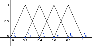
Imagine a degree 1 blending functions for $n=4$ curve. We have 4 control points, so we need 4 blending functions – triangular functions in the current case. There are 6 places where those functions start or end, these 6 values will be our knots for the blending functions.

When we have a higher degree blending functions, then there will be more knots. The number of knots is $n + d + 1$ and if we have uniform spacing, then they will divide the time range $[0, 1]$ into equal parts. There are cases, when some of those values will repeat or do not have an equal spacing.

Notice that we have been talking about the blending functions a lot here. Those blending functions are actually splines: they comprise of $d$ degree polynomials and 0 lines. As splines, they have knots in the endpoints (where the segments start and end). This is why our current curve is called a B-spline curve. The name means a basis-spline curve, basis functions is another name for the blending functions. Sometimes the curve part in the name is ommitted and a B-spline curve is just called a B-spline.

While 1st-degree blending functions are made up of lines, 2nd-degree blending functions are made up of parabolas. There are three distinct quadratic polynomials that form a $\text{C}^{~1} smooth spline at our knots.

This curve, although an approximating curve, has some nice properties:

• Any point on the curve is affected by at most $d+1$ blending functions, thus $d+1$ control points. So the control points will provide local control. You can see this if you look at the triangular functions. At any given time, there are at most 2 of those functions that have a non-zero value.
• We can achieve a high degree $n-1$ smoothness by doing the approximation with $d = n-1$ degree blending functions. This is the highest value we can use given $n$ points.
• We can also achieve lower degrees of smoothness. The degree is easily varied.
• There are even ways to get a lower degree of smoothness in only specific control points we want.

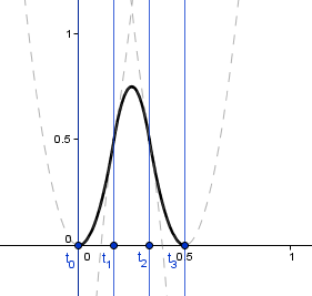
There is a problem, though, as you can see from the $n=4$, $d=1$ case, the ranges [0, 0.2) and (0.8, 1] have only one blending function. Even worse, it will tend to zero at 0 and 1. This means that the ranges [0, 0.2) and (0.8, 1] do not have enough support. If we were to vary the time $t \in [0, 1]$, then our curve would go to a point [0, 0, 0] at the ends. Now, one way would be to just take $t \in [0.2, 0.8]$ then. This will work and will give an approximating curve.

Another thing that we would want, would be that the curve would actually interpolate (connect with) the endpoints. The $d=1$ curve does that by itself, but higher degree curves will not. The range where they start to get the full support is after the time where the first blending function was at the maximum and others 0. Think about it, we need 3 blending functions together to calculate a point in a $d=2$ curve. Those three functions will start at different knots. When the last one starts, the second one already has some value, and the first one is past its maximum.

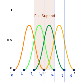
You can see all 4 of the blending functions there, but the full support is only in a limited range. We can correctly sample our curve only from that range.

In order to have full support in all of the $[0, 1]$ range, there is a technique to repeat the knots at the endpoints. Note that the new knot vector should be of the same length, but the 0 and 1 values are repeated $d$ times. This causes the blending functions to act in a way where we have full support over the entire unit range. This means that the curve passes the endpoints. You can try this out in the example on the right. The blending functions are drawn on the bottom-left corner.

Also, if we take the maximum degree of smoothness, e.g., with 8 control points, we can have a 7-degree polynomial which is $\text{C}^{~8}$ smooth. In that case, we actually get a Bezier curve.

You can see a more detailed explanation of how the blending functions are constructed here.

NURBS*

There is also an extension to B-spline curves called a NURBS (Non-Uniform Rational B-Spline) curve. As you saw before the knots uniformly distributed our time range $[0, 1]$. This does not have to be so, there can be a non-uniform distribution of knots. Only important thing is that it would be a monotonically increasing sequence.

The rational part of a NURBS curve comes from the fact that each control point can have a weight assigned to it. Those weights need to be normalized with a ratio and thus the name rational. The exact formula is as follows:

$C(t) = \dfrac{\sum_i B_{i, d}(t) \cdot w_i \cdot p_i}{\sum_i B_{i, d}(t) \cdot w_i}$

The vector $w$ is the vector of weights assigned to each control point. If the weights are all 1, then we have a normal B-spline. The example on the right allows you to try out different weights, although the knot vector is still left uniform.

NURBS curves are very often used to model all sorts of curves and surfaces. Not only are they affine invariant like the B-spline and Bezier curves, but if handled correctly, they are also correctly projected via a perspective projection.

You can read more about them (and other curves) here.