Noise

The source of all procedural generation is randomness. We are interested in creating algorithms that produce some reasonable system with a random behavior. Ok, so let us start with a function that gives random values. Note that the random number generators do not give true random values, but sample a function that will look like random. For simplicity it seems good to still call those values random, they could very well be.

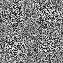
Unfortunately, if we look at random values, they will look back and appear as in the image on the right. So, how could we get something reasonable out of them?

One way would be to create a random spline through the noise values. That would be some spline that will interpolate our random values. The degree of smoothness does not matter much here. This is kind of the same if we were to just zoom in to the noise. There would not be new noise generated between the existing noise, but a transition would appear. With bilinear interpolation we have linear transitions, a $C^0$ spline.

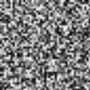
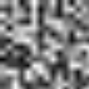
Below are some zoom levels of the previous noise image. 

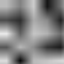x3	x9	x27

By themselves they do not seem much, but if we take a weighted sum of them, then the results are more interesting. 

This describes a technique called value noise. Take a set of random values in some dimension, interpolate between them. Do it with the values being more apart and more closer together (different frequencies) and sum the results.

There are actually many other things you could also do. Like I mentioned the weighted sum, depending on the application, this might not be needed. Some interesting patterns can be achieved by sending the result values to another function (like sine for example). Sometimes you would like to use some smoothing / blurring on the values.

On the right there is an example that implements one possibility. There are 6 different samples done on the original static noise image. The weights $weight_i$ define how much of the result we are considering in our sum. The zoom levels $zoom_i$ define how much are we zooming in to the texture. Or how far away the known values are in our random spline.

The result is a bit more scaled, because the noise texture was 128×128, but our window is 300×200. Do not let this bother you.

There are plenty of things this result pattern can be used for. You could:

• Use it as clouds texture (there is actually a tool called Clouds in some image manipulation programs that generate this pattern)
• Generate it on a sphere and call it a planet.
• Create marble or rusty metallic surface looks.
• Use it as a height map to generate some terrain.
• ...

For a good explanation in the 1D case I recommend to check out this page (they incorrectly say that it is Perlin noise). You can notice that in 1D it is sometimes much more important to create a smooth interpolation between the known random values: cosine and cubic interpolation are shown there besides the linear one.

Perlin Noise

Another way to generate a noisy pattern, is not to specify the values from random variables, but instead gradient directions. Even if we were to specify more smoother interpolations than just bilinear, for the value noise, the result would still be blocky. So, instead of value noise, we could create gradient noise instead.

The main idea behind gradient noise is, that we specify a gradient direction (instead of a value) for each grid point. We can assume, that the gradient has 0 at the grid point, and the direction vector points to the increasing direction. Part of a grid line would be something like this:

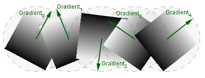
For simplicity we here assume, that all the random gradient directions are generated randomly from an unit circle. You can use a random choice from some predetermined fixed number of directions (specifying 8 or 12 different directions already would give a good result). Currently the gradient vectors are also normalized (come from an unit circle, like mentioned). You can try without normalizing them, then the results may vary.

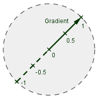
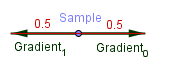
Now, given a grid of gradient directions, we want to sample a point between those grid points and interpolate between the values from the gradients. Notice, that each gradient defines its own plane. The center grid point has the value 0, and values increase towards the direction of the vector. In order to get a value for the sample point from the gradient plane, we can use our old friend, scalar projection.

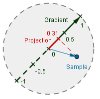We need to find the $Distance$ vector (blue) from the grid point to the sample point. Then, because the gradient vector is normalized, we can just find the value on the gradient as:

$value = |Distance| \cdot cos(∠(Distance, Gradient)) = Distance\cdot Gradient$

The values here can also be negative, which we need to take into account later on, when we want to display the result.

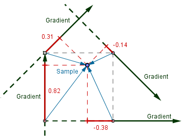
Now, we want to find the values on each of the 4 neighbouring gradient planes. Given those 4 neighbours, we find the corresponding distance vectors and do the scalar projection onto each of the gradient vector.

Lastly we want to interpolate between those 4 values to get the result. We can use bilinear interpolation here, but this will produce only a $C^0$ smooth spline like before. So there will be visible edges on the grid lines. When doing bilinear interpolation, there will actually be parabolae interpolating the 0 values at the grid point. This is because our interpolated value would be:

$value = (1-t) \cdot |Direction| \cdot \cos(\alpha) + t \cdot (1-|Direction|) \cdot \cos(\beta) = (1-t) \cdot t \cdot \cos(\alpha) + t \cdot (1-t) \cdot \cos(\beta)$

That equals: $(t - t^2)(cos(\alpha) + cos(\beta))$, so we have a parabola. The direction, where it opens, is determined by the angles between the different $Distance$ and the $Gradient$ vectors.

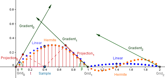
As you can see, there is a corner at $Grid_1$ with the linear interpolation (blue). Another way would be to use the blending function from the Hermite curve (orange). We use the Hermite blending function for the second control point from the Hermite curve, namely: $(3t^2 - 2t^3)$. This yields us also the complimentary polynomial $(1-3t^2 + 2t^3)$.

We can find out, how they behave in our case. So the interpolated value would be:
$value = (1-3t^2 + 2t^3) \cdot t \cdot \cos(\alpha) + (3t^2 - 2t^3) \cdot (1-t) \cdot \cos(\beta)$.

When we multiply with $t$, then we get:
$value = (t-3t^3+2t^4) \cdot \cos(\alpha) + (3t^2-5t^3+2t^4) \cdot \cos(\beta)$.
These two 4th order polynomials have the roots at $0$ and $1$, and are symmetric regard to the $x=0.5$ axis. They give us a smoother result for the noise. If you find the derivatives of that function on the end points, then you can see that they are $\cos(\alpha)$ and $\cos(\beta)$. This means that we have a $C^1$ smooth spline.

There is also a possibility to use a fifth order polynomial in the form $6t^5 - 15t^4 + 10t^3$, for even better result.

As mentioned before, some values can currently be negative, so for display purposes, we would need to convert our range into $[0..1]$. Because the gradient vector is normalized, then we can find out, that the extreme values are $-0.5$ and $0.5$. These are achieved, when we are on the center of a grid line and both the nearest neighbours are opposite of each other. The cosines are both $1$, we get $0.5$ (or $-0.5$) from the projection and the blending functions also give $0.5$.

For example, with $0.5$ we get $value = 0.5 \cdot 0.5 \cdot 1 + 0.5 \cdot 0.5 \cdot 1 = 0.25 + 0.25 = 0.5$

This means, that we can just add $0.5$ to the result, and we will be in the range $[0..1]$.

For the noise in higher dimensions the output range is $[-\frac{\sqrt{D}}{2}, + \frac{\sqrt{D}}{2}]$

On the right there is an example that does just that. You can try different interpolations, manipulate the zoom levels and weights just like before.

The gradient noise, just constructed, is called Perlin noise. I also recommend to check out Ken Perlin's slideshow on that topic, and also this site, that describes both value and gradient noise.

L-Systems

Some objects we would want to have are self-similar. Consider a tree for example. It starts from the trunk and then branches out. At some point along the branch there is another branching, then another branching and so on. We have a specific notion of branching there, although the actual direction of the branch and the point where it occurs, may vary.

You might have learned about formal grammars in a program code translation course. Code of a program is also somehow self-similar (we can have if-statements inside if-statements etc). Here however we will not use formal grammars to analyze a written code, but the other way around. From a formal grammar we can also derive all of the words expressible in that grammar.

Simply put, grammar is a set of rules. Each rule has a left side and a right side. Here we consider context free grammars, where a rule can be applied by matching the left side and not considering what is before or after the left side in our word. 
Consider just this rule:

$\text{F} \rightarrow \text{FF}$

We can derive arbitrary sequences of $\text{F}$-s with that, when we start with just a word $\text{F}$. The starting word is called an axiom.

In order to determine a derivation, we will do parallel rewriting. This means that we consider the current word and rewrite all of the terms in it at once. With out current example we would only get the sequences:

$\text{F}$ - no iteration

$\text{FF}$ - 1st iteration

$\text{FFFF}$ 2nd iteration

$\text{FFFFFFFF}$ 3rd iteration

...

This means that we will get a fixed word after a number of iterations via parallel rewriting. We want to have a specific result after a specific number of iterations. However we would want some variation in what the actual result will be. We will see why in a moment.

First let us think, how this actually helps us to generate anything? The key is in the interpretation of the word. Consider the following rule:

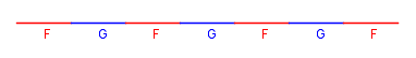
$\text{F} \rightarrow \text{FGF}$

Notice that now we will get a term $\text{G}$ in our word, but we do not have a rule for $\text{G}$ defined. Usually the identity rule is assumed to exists in such a case. So this means that after the 2nd iteration, we get:

$\text{FGFGFGF}$

Now, we can start interpreting that word. Let us say, that whenever we have $\text{F}$, we will draw a red line from the current position and move the current position at the end of that line. When we have G, we will draw a blue line and move to the end of that.

Now, if we consider trees, then we would want to have some sort of branching. For this, we would need to remember the position in the beginning of the branching and return to it after the branch has ended. This is quite similar to tree data structure representation. We will use square brackets to specify the beginning and end of a branch. We need one more thing, a branch should change the orientation. Let us use the $\text{+}$ symbol to denote a fixed rotation. Consider now the following rule:

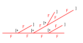
$\text{F} \rightarrow \text{F[+F]F}$

After the 2nd iteration from $\text{F}$ we have:

$\text{F[+F]F[+F[+F]F]F[+F]F}$

When we interpret it, we get:

These all already sufficient building blocks to generate self-similar objects. Although, given a grammar and the iterations count, we will always get the same object. In order to provide more variety, we can make the grammar stochastic. This means that each rule has a certain probability attached to it. There can now be many rules with the same left side, but the sum of the probabilities of those must be 1. Otherwise it may happen that no rule will get applied. Of course we could consider that in that case we apply the identity rule, but that might not be that transparent.

So a stochastic grammar would look something like:

$\text{F} \xrightarrow{0.5} \text{F[+F]F}$

$\text{F} \xrightarrow{0.5} \text{FGF}$

At each rewriting step for $\text{F}$ we will consider both of those rules and pick one according to their probabilities.

This is called a stochastic context free Lindenmayer-system. Aristid Lindenmayer was a botanic who created these kinds of systems when studying the self-similarity in plants. You can read more about it in his paper The Algorithmic Beauty of Plants, that has also plenty of examples.

The example on the right uses following ruleset:

$\text{B} \xrightarrow{p_0} \text{C[^B[+B][-B]]}$

$\text{B} \xrightarrow{p_1} \text{C[&B[^B][-B]]}$

$\text{B} \xrightarrow{p_2} \text{C[-B[+B][&B]]}$

$\text{B} \xrightarrow{p_3} \text{C[+B][-B]}$

The symbols $\text{+}$, $\text{-}$, $\text{^}$ and $\text{&}$ denote to positive and negative rotations around the x and z axes. There is a 10° randomness around 30° rotation for each of them. Terms $\text{B}$ and $\text{C}$ denote that we should draw a branch from the current location. Term $\text{C}$ will not change in any subsequent iterations.

You can see what happens when you change the probabilities of those rules. For example change the probability of the last rule ($p_3$) to be equal to 1. Then you will not have a stochastic system anymore and you can see that the result is always the same general shape.

A good thing about this kind of approach is that you can easily change how your tree looks like, if you change the probabilities or rules. This provides a common framework for creating many different self-similar objects. 

Particle Systems

Another way of generating effects is via a particle system. Now, you can have all sorts of objects act as particles, for example you might have modeled a bubble and now want many of them spawning from a fountain full of soap and bursting after some time. Traditionally a particle system will have very small objects as particles and there will be a lot of them. Together they will make up a fancy effect.

Depending on the needs, there will be different components in a particle system. Here we present a really simple one.

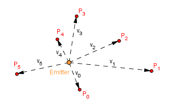
First we have an emitter, where all the particles spawn. This emitter can just be a location in your space. All of the particles start from that location and move in some trajectory. In our example each particle will pick a random direction in which it will move. There will also be random speed for each particle, random from some range that is. We can call the trajectory + speed a velocity and denote it $v_i$.

Now, the particles will continue to spawn from the emitter with some rate and travel with their velocity (unless other forces change it). After some time a particle may die. We can call this time the time to live. If that time has passed from the particle's spawn, then we remove the particle. Otherwise our all scene will be filled with particles and more continue to spawn.

There might be some effects we want to do, when a particle reaches the end of its life. For example we can increase the opacity to make it seem to fade away. We might also change the color or play the bursting animation if it is a bubble. In the current example we just decrease the opacity when there is a decay number of milliseconds left for the particle to live.

A good programming pattern to use here is a worker pool pattern. We create a pool of particles when we create the emitter. When a particle dies, it returns to the pool and becomes available to spawn again. This of course assumes that we have a big enough pool. If you change the particle's lifetime to first into very small value and then to a too large value, then you can see a pulsating effect from the emitter. This happens because the particle pool becomes empty. Particles live longer, there are more of them in the scene at once.

But you do not have to have an emitter and particles constantly spawning and dying. There might already be a number of particles visible and we want some kind of behavior assigned for them. Previously we just had a random velocity for the particles.

There is an algorithm called Boids that tries to mimic the flocking of birds. It is a particle system that follows a couple of simple rules:

• Cohesion – Each particle tries to move towards the center of mass of all the particles. If the mass is the same, then we can sum all of the positions and find the average of them to get the center of the mass.
• Separation – Each particle tries to avoid other particles. If it becomes too close to one, it will move away from it.
• Alignment – Each particle tries to follow the average velocity of other particles. This is quite similar to the center of mass, we sum all the velocities and find the average.

Those are the basic rules. Of course one can add more rules to those. For example the particles might try to follow some moving target. Or they might collide with walls or avoid obstacles. 

There are many versions and additions to this algorithm. More explanation can be found here and here.