Geometry and Transformations II
Previously we saw some linear transformations: scale, rotation and shear. Unfortunately those are quite limiting transformations. For example if we want to rotate an object around its center, the center should be located in the origin. We do not want all of our objects in our scene to be located in the origin though. The origin will of course be somewhere in our world space, but other objects might be located at coordinates $(10, 40, 25)$ or $(-30, 100, 0)$. So how do we get those objects there?
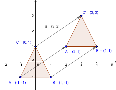
With linear transformations new coordinates will always depend on the values of the previous coordinates. We would however add a scalar value to the coordinates. For example we might start out with a triangle whose vertices are $(1, 1)$, $(0, 1)$ and $(-1, -1)$. We might even do some transformation to it like scaling and rotation, because it is in some way centered in the origin. But before actually rendering it, we want to add some shift to all of the coordinates.
Here are some definitions that we look at during this chapter:
- Translation – a transformation that will add a scalar value to the coordinates.
- Affine transformation – a transformation that will preserve parallelness of parallel lines.
- Commutativeness – property of an operation where the order of operands does not change the result.
- Associativity – property of an operation where the the order of consecutive operations does not change the result: $(a \cdot b) \cdot c = a \cdot (b \cdot c)$
- Scene graph – a graph (usually a tree) that defines the relations between objects (that may be abstract) in a scene.
- Stack – a data structure that has the push() and pop() operations. Push will add a value to it, pop will return the last added value.
Translation
This is where the homogeneous coordinates and the shear operation tie together to allow for translation and thus affine transformations. It is useful to distinguish that an affine transformation may not be linear any more, i.e. does not satisfy the linearity property. This will become more clear, when we look at one way to construct the translation.
For this construction, imagine a very simple 1D world, where everything is located at a $y=1$ line:
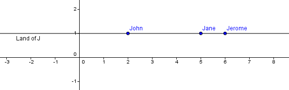
All of those objects have a single coordinate in their 1D world.
$John = (2)$, $Jane = (5)$, $Jerome = (6)$.
We could do the scaling linear transformation on it, if we want. This would be identical to scalar multiplication, because our transformation matrix would be of size 1×1.
But we can look at this world in a one dimension higher space, the 2D space. In that higher space, the coordinates would be:
$John = (2, 1)$, $Jane = (5, 1)$, $Jerome = (6, 1)$.
This looks a lot like homogeneous coordinates that we have talked before, and actually it is just that. In this higher space we could also perform some transformations. As you might notice, rotation and scaling will generally move our objects out of the 1D world located at $y=1$. But we could try the shear-y operation, that will keep the y coordinates the same, but tilts the y axis, thus changing the x coordinates.
We will do the shear-y with 45°, because $tan(45°) = 1$.
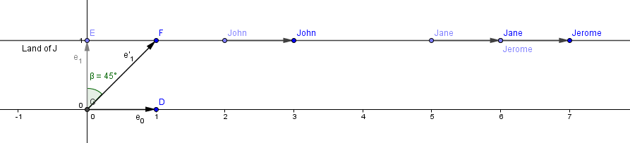
As you can see, all our points have moved 1 unit to the right (positive x direction). The general matrix for the shear-y would be:
$ \left( \begin{array}{cc}
1 & shearY \\
0 & 1
\end{array} \right)
\left( \begin{array}{cc}
x \\
1
\end{array} \right) =
\left( \begin{array}{cc}
x + 1 \cdot shearY \\
1
\end{array} \right)
$
This is exactly what we want. We want to add a coordinate-independent scalar value to the corresponding coordinate of each of our points.
Next we do not have to care about the exact angle we use for the shear. We can just put our desired translation value in the corresponding position. For higher spaces the construction is the same. We will go to one dimension higher space and do the corresponding shear operation there.
This will give us an augmented transformation matrix that represents affine transformation (linear transformation + translation). In 3D it would be:
$ \left( \begin{array}{cc}
a & b & c & translateX \\
d & e & f & translateY \\
g & h & i & translateZ \\
0 & 0 & 0 & 1
\end{array} \right)
$
The letters $a, b, ..., i$ will represent the linear transformation part; last column is called the translation column and the last row should always be $(0, 0, 0, 1)$. Later we can see that some of the values in the last row can be used for a perspective projection transformation, but for your usual affine transformations you should not change it.
Consider the example on the right. I have positioned the vertices to be at coordinates $(1, 1, 1)$, $(-1, 1, 1)$, $(-1, -1, 1)$, $(1, -1, 1)$. So we have a 2D world located at $z=1$ plane in 3D space. In order to do the shear-z operation in 3D, we need two values: how much shear on the x direction and how much on the y direction. Those two values are in the translation column.
As you might have guessed by now, the reason for a 4×4 matrix is that in 3D space, if we want to do the translation, we need to go to a 4D space and shear there.
Multiple Transformations
Natural question arises here, that how can we do multiple transformations? For example if we want to rotate our object and then translate it. Or perhaps we want to translate it and then rotate? Will there even be a difference?
One can probably figure out that we can construct multiple transformation matrices and then apply them sequentially: using the next one on the results of the current one. Note that matrix multiplication is associative and we can regard our column-vectors as matrices with width 1. Because of that we could multiply our transformations together and after that do only one matrix-vector multiplication for each of our vertices.
In other words, suppose that we have transformation matrices $T_1$, $T_2$ and $T_3$. Our vector will be $v$. Of course, in practice, this transformation will be applied to all of the vertices you have sent to the GPU in the vertex shader.
$T_1 (\cdot T_2 (\cdot T_3 \cdot v)) = (T_1 \cdot T_2 \cdot T_3) \cdot v$.
As you can see, we can multiply the transformations together once before transforming any of the vertices. After that, we can do just one matrix-vector multiplication in the shader. Instead of sending 3 (or more) transformation matrices and doing a number of the same matrix-matrix multiplications for all of the vertices. This matrix is usually called the model matrix and denoted $M$ as it encompasses all the transformations relative to a single 3D model (object).
In other words:
$M = T_1 \cdot T_2 \cdot T_3$
We send to the vertex shader the matrix $M$ and our vertex set $V$. Let $v \in V$, in the vertex shader for each $v$ we only do:
$M \cdot v$.
Still, as you know, matrix multiplication is not commutative. This means that the order we apply the transformations, generally makes a difference. There is a different result depending on do we say that $M = T_1 \cdot T_2 \cdot T_3$ or perhaps $M = T_3 \cdot T_2 \cdot T_1$.
Very simple example would be to do the rotation and translation. Let us rotate 90° around the z axis and translate by a vector $(1, 2, 0)$.
$ \left( \begin{array}{cc}
0 & -1 & 0 & 0 \\
1 & 0 & 0 & 0 \\
0 & 0 & 1 & 0 \\
0 & 0 & 0 & 1
\end{array} \right) \cdot
\left( \begin{array}{cc}
1 & 0 & 0 & 1 \\
0 & 1 & 0 & 2 \\
0 & 0 & 1 & 0 \\
0 & 0 & 0 & 1
\end{array} \right) \cdot
\left( \begin{array}{cc}
x\\
y \\
z \\
1
\end{array} \right) =
\left( \begin{array}{cc}
0 & -1 & 0 & -2 \\
1 & 0 & 0 & 1 \\
0 & 0 & 1 & 0 \\
0 & 0 & 0 & 1
\end{array} \right) \cdot
\left( \begin{array}{cc}
x\\
y \\
z \\
1
\end{array} \right) =
\left( \begin{array}{cc}
-y - 2\\
x + 1 \\
z \\
1
\end{array} \right) $
If we apply the transformations the other way:
$
\left( \begin{array}{cc}
1 & 0 & 0 & 1 \\
0 & 1 & 0 & 2 \\
0 & 0 & 1 & 0 \\
0 & 0 & 0 & 1
\end{array} \right) \cdot
\left( \begin{array}{cc}
0 & -1 & 0 & 0 \\
1 & 0 & 0 & 0 \\
0 & 0 & 1 & 0 \\
0 & 0 & 0 & 1
\end{array} \right) \cdot
\left( \begin{array}{cc}
x\\
y \\
z \\
1
\end{array} \right) =
\left( \begin{array}{cc}
0 & -1 & 0 & 1 \\
1 & 0 & 0 & 2 \\
0 & 0 & 1 & 0 \\
0 & 0 & 0 & 1
\end{array} \right) \cdot
\left( \begin{array}{cc}
x\\
y \\
z \\
1
\end{array} \right) =
\left( \begin{array}{cc}
-y + 1\\
x + 2 \\
z \\
1
\end{array} \right) $
As you can see, the rotation will rotate our geometry to be the same in both cases, but the actual translation will take the object to different places. You can think about two cases:
- First rotating the geometry in place and then translating it.
- First translating the geometry to a new location and then rotating it.
You can try it out in the example on the right. Try choosing different order for the translation and rotation. Then change the translation values (for x and y) and the $\alpha$ for the rotation angle.
Keep in mind that the transformations are applied from right to left. The matrix near the vertex is applied first. So if the rotation matrix is the right-most, then the vertices are first rotated and then translated. If the translation matrix is the right-most, then the vertices are first translated and then rotated (around the origin).
Matrix Stack
Besides applying multiple transformations to a single object, we might also have multiple objects in our scene with different transformations. There might be a dependency between the transformations of some objects. For example, what if we have triangles that should rotate around another triangle?
In the next chapter we will see more about frames of reference, but the idea is that there are actually many coordinate systems. As you might have seen from the previous example, if we do the rotation before the translation, the rotation occurs around the initial origin. When we change the rotation, then in the result the triangle visually rotates around a different origin. Technically the rotation still occurs around the initial origin and the object is then translated, but mathematically you can also think that we have first shifted the origin and then rotating around another origin ($O'$). So the moved triangle actually has a different frame of reference (coordinate system).
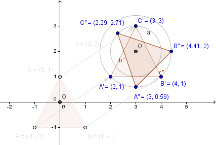
Consider the example on the right. We have a big triangle and two smaller ones. There is notion of a scene graph there that defines the smaller triangles to be children of the first one. When parsing the scene graph, we want to save our intermediary matrices because we need to come back to them after a branch has been parsed.
We do not want to have variables for all the possible matrices, rather we want a single matrix, that we will multiply in order to represent the current transformation. Consider the following:
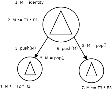
- We first have our transformation matrix M set to identity (no transformation).
- We multiply it from the right with the translation (T1) and rotation (R1) of the big triangle.
This matrix (M = T1 * R1) is applied to the vertices of the big triangles. - We push this matrix to a matrix stack for later use.
- We multiply the current transformation matrix from the right with the translation (T2) and rotation (R2) of the first smaller triangle.
This matrix (M = T1 * R1 * T2 * R2) is applied to the vertices of the first smaller triangle. - We need the matrix we saved in step 3, we will pop it from the stack.
- We push this matrix to a matrix stack for potential later use again.
- We multiply the current transformation matrix from the right with the translation (T3) and rotation (R3) of the second smaller triangle.
This matrix (M = T1 * R1 * T3 * R3) is applied to the vertices of the second smaller triangle. - We pop the saved matrix from the stack.
You see that the transformation matrix of the big triangle is used 3 times (the T1 * R1 part). Using the stack, we can calculate it once and before changing it, save it to the stack for later use. We use the stack, because there might be more levels than just 2 in the scene graph and there might be more intermediary matrices that need to be saved and reused.
Rotation Revisited*
We saw how rotation can be represented by a rotation angle around some axis. For rotation around an arbitrary vector, we mentioned that we can first rotate that vector to be an axis, do the rotation around the axis, and reverse the initial rotation. This works for the simple cases, but there is a problem called a gimbal lock. Depending on the order in which we apply the rotation around x, y and z axes, we might lose a degree of freedom. This happens when we store the rotations as three angles (called Euler angles) and use corresponding matrices to transform the geometry. Furthermore the transition from one rotation to another might experience weird behavior.
Gimbal Lock
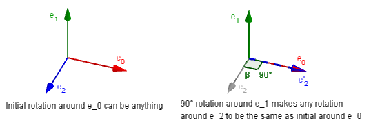
The gimbal lock problem can occur, when you have defined the rotation of some object by the Euler angles. Those 3 rotation values need to be applied in some order in which they are applied. For example if the order is defined as XYZ, then the rotation is defined as:
- Rotate around X
- Rotate around the transformed Y (rotated by step 1)
- Rotate around the transformed Z (rotated by steps 1 and 2)
This is because the rotation will be applied in the space you are currently in. After step 1. you have already changed the space. If you happen to rotate exactly 90° around Y in step 2, then the Z axis will be aligned with the original X and you have lost a degree of freedom.
The example on the right shows exactly that. You can choose the order of your Euler angles, which define the rotation of the object and then press Lock to align the first and third axes.
Axis Angle (Rodrigues' Rotation Formula)
As we saw, defining the rotation of an object by the Euler angles has the problem of gimbal lock. That is not the only problem and thus there is valid reason to try some other representation. Any orientation of an object can be defined by using an axis of rotation and an angle (the amount rotated on the given axis).
Let us investigate how rotating around an arbitrary axis works. We do know from before that we could rotate that axis to be aligned with one of the basis vectors, rotate around that, and then inverse the alignment. That is quite a long way to do a simple rotation (includes finding several matrices, their inverses and then multiplying them all together).
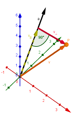
First thing to notice about rotating a point $P$ around an axis $a′$ is that the location vector $v$ of the point can be decomposed into two components: the vector parallel to the axis - $v_{∥}$, and the vector perpendicular to the axis - $v_{⊥}$.
This means that $v = v_{∥} + v_{⊥}$.
To get the parallel vector you can take the scalar projection of $v$ onto $a$. For that we need a normalized $a′$, call it $a = \frac{a′}{||a′||}$.
So $v_{∥} = a \cdot (a \cdot v)$.
Finding the perpendicular vector is easy as doing $v_{⊥} = v - v_{∥}$.
Note that the only the perpendicular component will actually change when we rotate around the axis of rotation. The parallel will stay the same.
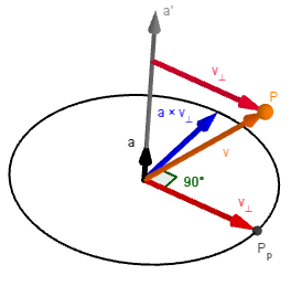
For the next step we find a vector orthogonal to $v_{⊥}$, which has the same size and is located in the positive direction.
As can be seen from the illustration on the left, we need the normalized axis $a$ for that.
We can use the cross product to find the vector: $a × v_{⊥}$.
The reason for it is that we want to find new coordinates for the rotated vector $v$, so we need two linearly independent vectors for it. The orthogonal ones are the easiest.
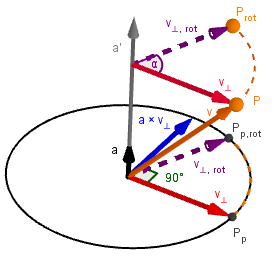
Here you can see the actual rotation of $P$ to $P_{rot}$.
Notice that $||v_{⊥}|| = ||v_{⊥,rot}|| = ||a × v_{⊥}||$.
The origin of the vectors on this illustration does not matter. I have drawn the $a × v_{⊥}$ to start from the same place where $a$, but actually you could also place them to the point where $v_{⊥}$ intersects $a$ on the illustration. Whichever way you want to imagine it.
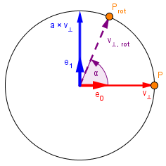
Next we have two ways we can approach this. Both look at the plane perpendicular to the axis of rotation.
| Approach 1 | Approach 2 |
|---|---|
|
In the first approach you could define a orthonormal basis with the two perpendicular vector we have. The basis vectors will just be the normalized: $e_0 = \frac{v_{⊥}}{||v_{⊥}||}$ $e_1 = \frac{a × v_{⊥}}{||v_{⊥}||}$
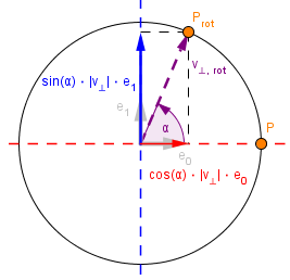
Next you can find the coordinates of the rotated vector by looking at the definitions of trigonometric functions sine and cosine. If you have found the coordinates then to get the actual rotated vector, just take a linear combination with the basis vectors. $v_{⊥,rot} = \cos(\alpha) \cdot || v_{⊥} || \cdot e_0 + \sin(\alpha) \cdot || v_{⊥} || \cdot e_1$ If you substitute the basis vectors, then the equation simplifies to: $v_{⊥,rot} = \cos(\alpha) \cdot v_{⊥} + \sin(\alpha) \cdot (a × v_{⊥})$ |
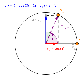
Another approach would be to take the vector projection of the rotated vector to the orthogonal vectors. Vector projection is a scalar projection multiplied by the normalized vector projected onto. If we put the formulas together they simplify here: $v_{red} = \frac{v_{⊥}}{||v_{⊥}||} \cdot (\frac{v_{⊥}}{||v_{⊥}||} \cdot v_{⊥,rot}) = $
$v_{blue} = \frac{a × v_{⊥}}{||v_{⊥}||} \cdot (\frac{a × v_{⊥}}{||v_{⊥}||} \cdot v_{⊥,rot}) = $
If you add those two together, you come to the same result as with Approach 1: $v_{⊥,rot} = \cos(\alpha) \cdot v_{⊥} + \sin(\alpha) \cdot (a × v_{⊥})$ |
With that result then final formula for the rotated point will be:
$v_{rot} = v_{∥} + v_{⊥,rot} = a (a \cdot v) + \cos(\alpha) v_{⊥} + \sin(\alpha) (a × v_{⊥}) = a (a \cdot v) + \cos(\alpha) (v - a \cdot (a \cdot v)) + \sin(\alpha) (a × v_{⊥})$
There is one more simplification we can do with the last cross product:
$a × v_{⊥} = a × (v - v_{∥})$
Because of the cross product's distributivity over addition:
$a × (v - v_{∥}) = a × v - a × v_{∥} = a × v - 0$
So now the final final result to rotate any point $v$ around axis $a$ by angle $\alpha$ is:
$v_{rot} = a (a \cdot v) + \cos(\alpha) (v - a (a \cdot v)) + \sin(\alpha) \cdot (a × v)$
This should be quite easy for the computer to calculate, only one unique dot product, one cross product, 2 trigonometric functions, lastly a few multiplications and additions. This result is named Rodrigues' rotation formula and it is implemented in your usual rotateAxisAngle() methods.
On the right you have an example, where you can define an axis and then rotate the object around it. Notice that all different rotations can be achieved from the initial 0 rotation with just these 4 values.
Quaternions
As we saw the axis-angle representation is quite good to hold the object's rotation. It will however have some shortcomings if we want to change the object's rotation by some other rotation. Or to smoothly interpolate the rotation between two fixed rotations. Thus enter quaternions.
Quaternions are elements of a number system beyond complex numbers. Instead of one imaginary unit $i$ they also have $j$ and $k$. The math works similarly to the complex numbers, but includes more terms. There are also important rules for multiplying the imaginary terms.
With your ordinary complex units we have $\sqrt{-1} = i$ thus $i^2 = -1$. Here the same thing applies for also $j$ and $k$. Meaning: $i^2 = j^2 = k^2 = -1$. Furthermore there are rules for what happens if we multiply together the imaginary units. The following table is read from row to column. So for example the first row tells that $ij = k$ and $ik = -j$:
| $ \cdot $ | $i$ | $j$ | $k$ |
|---|---|---|---|
| $ i $ | $ -1 $ | $ k $ | $ -j $ |
| $ j $ | $ -k $ | $ -1 $ | $ i $ |
| $ k $ | $ j $ | $ -i $ | $ -1 $ |
A quaternion can be written with 4 coordinates:
$q = (a, b, c, d) = a + bi + cj + dk$
Often the real part is separated and the imaginary part is called the vector part. In that case the vector part is represented as a vector $v = (v_x, v_y, v_z) = (b, c, d)$. Thus a quaternion can also be written as:
$q = (a, v)$
In order to use quaternions for rotation we need to represent two things:
- Our vectors (which we rotate) will be pure imaginary quaternions. If we want to rotate a vector $v$, then we need to create a quaternion $v = (0, v)$
- The axis $a$ and the angle $\alpha$ will be represented as a quaternion $q = (\cos(\frac{\alpha}{2}), \sin(\frac{\alpha}{2})a)$
If we do that, then we can rotate a vector by multiplying its quaternion representation by $q$ from the left and its inverse $q^{-1}$ from the right.
$v_{rot} = qvq^{-1}$
An important thing to note here is that the quaternion representing the rotation needs to be an unit quaternion. This means that our axis vector $a$ needs to be normalized. If it is, then it is easy to check that:
$\cos^2(\frac{\alpha}{2}) + \sin^2(\frac{\alpha}{2})||a|| = \cos^2(\frac{\alpha}{2}) + \sin^2(\frac{\alpha}{2}) \cdot 1 = 1$
As $q$ is a unit quaternion its inverse will be its conjugate $q^{-1} = q^* = (\cos(\frac{\alpha}{2}), -\sin(\frac{\alpha}{2})a)$
So let us see what happens if we perform the mentioned multiplication. One has to be careful here, because multiplying the vector parts of quaternions (or just quaternions) is non-commutative. This is logical because for example $ij \neq ji$.
$qvq^{-1} = (\cos(\frac{\alpha}{2}) + \sin(\frac{\alpha}{2})a)v (\cos(\frac{\alpha}{2}) - \sin(\frac{\alpha}{2})a) = $
$~~~~~~~~~~ = (\cos(\frac{\alpha}{2})v + \sin(\frac{\alpha}{2})av)(\cos(\frac{\alpha}{2}) - \sin(\frac{\alpha}{2})a) = $
$~~~~~~~~~~ = \cos^2(\frac{\alpha}{2})v + \sin(\frac{\alpha}{2})\cos(\frac{\alpha}{2})av - \sin(\frac{\alpha}{2}) \cos(\frac{\alpha}{2})va - \sin^2(\frac{\alpha}{2})ava = $
$~~~~~~~~~~ = \cos^2(\frac{\alpha}{2})v + \sin(\frac{\alpha}{2})\cos(\frac{\alpha}{2})(av - va) - \sin^2(\frac{\alpha}{2})ava$
This is a pretty result, but does not tell much yet. In order to simplify it, we need to derive some identities with pure imaginary quaternions. So what happens if we multiply $av$?
$av = (a_xi + a_yj + a_zk)(v_xi + v_yj + v_zk) = $
$~~~~ = a_x v_x ii + a_x v_y ij + a_x v_z ik + a_y v_x ji + a_y v_y jj + a_y v_z jk + a_z v_x ki + a_z v_y kj + a_z v_z kk = $
$~~~~ = -a_x v_x + a_x v_y k - a_x v_z j - a_y v_x k - a_y v_y + a_y v_z i + a_z v_x j - a_z v_y i - a_z v_z = $
$~~~~ = (-a_x v_x - a_y v_y - a_z v_z) + (a_y v_z - a_z v_y) i + (v_x a_z - a_x v_z) j + (a_x v_y - v_x a_y) k = $
$~~~~ = - a \cdot v + a × v = a × v - a \cdot v$
This gives us a quaternion, where the vector part can be found by taking the cross product and the real part by taking the negative dot product. So simplifying the middle term $av - va$ should be really easy:
$av - va = a × v - a \cdot v - v × a + v \cdot a = a × v - a \cdot v + a × v + a \cdot v = 2(a × v)$
To simplify the last term $ava$ we need two preliminary identities.
- $av = a × v - a \cdot v = - v × a + a \cdot v - 2a \cdot v = -va - 2(a \cdot v)$
- $aa = a × a - a \cdot a = - a \cdot a$
Now to simplify:
$ava = (-va - 2(a \cdot v))a = -vaa - 2(a \cdot v)a = (a \cdot a)v - 2(a \cdot v)a = v - 2(a \cdot v)a$
If we substitute those back in the original result we can continue:
$qvq^{-1} = \cos^2(\frac{\alpha}{2})v + \sin(\frac{\alpha}{2})\cos(\frac{\alpha}{2})(av - va) - \sin^2(\frac{\alpha}{2})ava = $
$~~~~~~~~~~ = \cos^2(\frac{\alpha}{2})v + 2\sin(\frac{\alpha}{2})\cos(\frac{\alpha}{2})(a × v) - \sin^2(\frac{\alpha}{2})(v - 2(a \cdot v)a) = $
$~~~~~~~~~~ = \cos^2(\frac{\alpha}{2})v + 2\sin(\frac{\alpha}{2})\cos(\frac{\alpha}{2})(a × v) - \sin^2(\frac{\alpha}{2})v + 2\sin^2(\frac{\alpha}{2})(a \cdot v)a = $
$~~~~~~~~~~ = (\cos^2(\frac{\alpha}{2}) - \sin^2(\frac{\alpha}{2}))v + 2\sin(\frac{\alpha}{2})\cos(\frac{\alpha}{2})(a × v) + 2\sin^2(\frac{\alpha}{2})(a \cdot v)a$
Next we need to remember couple of trigonometric identities:
- $\cos^2(\frac{\alpha}{2}) - \sin^2(\frac{\alpha}{2}) = \cos(\alpha)$
- $2\sin^2(\frac{\alpha}{2}) = 1 - \cos(\alpha)$
- $2\sin(\frac{\alpha}{2})\cos(\frac{\alpha}{2}) = \sin(\alpha)$
Using those we get:
$qvq^{-1} = (\cos^2(\frac{\alpha}{2}) - \sin^2(\frac{\alpha}{2}))v + 2\sin(\frac{\alpha}{2})\cos(\frac{\alpha}{2})(a × v) + 2sin^2(\frac{\alpha}{2})(a \cdot v)a) = $
$~~~~~~~~~~ = \cos(\alpha)v + \sin(\alpha)(a × v) + (1 - \cos(\alpha))(a \cdot v)a) = $
$~~~~~~~~~~ = \cos(\alpha)v + \sin(\alpha)(a × v) + (a \cdot v)a) - \cos(\alpha)(a \cdot v)a) = $
$~~~~~~~~~~ = (a \cdot v)a + \sin(\alpha)(a × v) + \cos(\alpha)(v - (a \cdot v)a)$
If you compare that to the Rodrigues' rotation formula derived in the previous section, then you can see that it is identical. Thus rotation is done by doing the multiplication $qvq^{-1}$, where $v$ is a pure imaginary quaternion representing a location vector and $q$ is a quaternion in the form $q = (cos(\frac{\alpha}{2}), sin(\frac{\alpha}{2})a)$ and $a$ is the unit vector of rotation.
With this representation if you want to apply multiple rotations then it is as simple as multiplying the previous result again the same way. So if we have quaternions $q_1$ and $q_2$ then:
$v_1 = q_1 v_0 q_1^{-1}$ followed by $v_2 = q_2 v_1 q_2^{-1}$.
If you write them together you get: $v_2 = q_2 q_1 v_1 q_1^{-1} q_2^{-1}$.
From this you can see that instead of always multiplying some $v$ you could instead multiply the quaternions together, because quaternion multiplication is associative. Here you can combine $q = q_2 q_1$ and then you can do again just $v_{rot} = qvq^{-1}$ and that operation has combined both of the rotations we defined as quaterions.
In practice the orientation of an object is usually held as a quaternion and if the rotation is changed, another quaternion is multiplied to the previous one. When rendering the final quaternion is converted into a rotation matrix, which is then sent to the GPU.
On the right there is an example, which shows the quaternion, when the object rotates. The rotation here is achieved by slerping between two quaternions. We will discuss this in the next section.
Quaternion Animation & Slerp
Often times you want to interpolate from one rotation to another. For example you know the target rotation (axis and angle) how an object should be, but just snapping to that rotation will look unrealistic in your application. Then you want to move somewhat towards your target rotation each frame (depending on the passed time of course). With translation and scale that could be achieved by just linearly interpolating (lepring) between the current and target value. With rotation, however, linear interpolation of the Euler angles would not give the best result: you will get to the target, but the path taken there is generally ill (not the shortest, does weird curves etc).
This is why with quaternions one can do spherical linear interpolation (slerp). This will ensure that the axis of orientation moves along a sphere and takes the shortest path. The formula for slerping between some initial rotation $q$ and the target rotation $p$ would be:
$r = \frac{q(\sin[(1-t)\theta]) + p\sin(t\theta)}{\sin(\theta)} = \frac{\sin[(1-t)\theta]}{\sin(\theta)}q + \frac{\sin(t\theta)}{\sin(\theta)}p$.
The angle $\theta$ is the half-angle between the quaternions $q$ and $p$. Value $t$ is the time from $0$ to $1$. If this interpolation is done for all the elements of the quaternion, then the resulting interpolated rotation will be smooth across a sphere.
More info here.
On the right there is an example, where you can set the target rotation and see the difference between lerping Euler angles and slerping quaternions. Notice that depending on the orientation, the actual axis may change the direction and angle will then change the sign. This is especially useful with quaternions as the shortest rotation may be by doing just that. The Euler angle representation is unstable in that regard, meaning that it may try to go the long way. For example interpolate the rotation so that the positive direction will be aligned with the target, when in reality the shortest way would be to align the negative direction and negate the angle.
Slerp is very often used in computer graphics for changing object's rotation.