Depth Buffer

Depth buffer (also known as z-buffer) is a way to keep track of the depth of every pixel (fragment) on the screen. The buffer is usually arranged as a 2D array with one integer value for each screen space pixel. The depth value is proportional to the distance of the fragment that has been drawn. However there is a lot of precision close to the camera and very little off in the distance. 

In the projection chapter we saw how the $z'$ value is calculated using projection matrix. This value was in range $[-1, 1]$ where -1 corresponds to the near plane and 1 to the far plane. The corresponding equation is: (z is the fragment distance from camera)

$z' = \dfrac{far + near}{far - near} + \dfrac{1}{z}\cdot \left ( \dfrac{-2 \cdot far \cdot near}{far - near} \right )$

In order to store this value in the depth buffer it is first normalized into to range [0, 1] by substituting conversion:

$z'_2 = \dfrac{(z'_1 + 1)}{2}$

Then it is multiplied by the max value of our depth buffer ($maxval=2^d-1$, where $d$ is the size of the depth buffer, usually 32 bits) and rounded to an integer. Resulting value is stored in the depth buffer.

While objects are rendered one by one the complete image is stored in the framebuffer. The framebuffer has its own depth buffer to keep track on z values of each already drawn pixel. Depth test is performed when new portion of geometry is processed (by vertex and fragment shader) and ready to be drawn to the framebuffer. Depth test compares each pixel z value to the corresponding pixel value in the framebuffer. If it is bigger the new pixel value is discarded otherwise it is overwritten or blended together (depending on whether blending is enabled or not).

Sometimes the source and the destination pixels happens to have exactly the same value. This problem was more common on older video cards because they had smaller depth buffer resolution, however it can also appear in current games with very large sight distance. The overall effect is annoying flickering that is called z-fighting. This effect can be avoided by reducing the depth of our view frustum and careful modelling of the distant geometry.

Color Blending

Color blending is a way to mix two colors together to produce to third color. These colors are called source and destination and they are in form $[R, G, B, A]$ where $R,G,B,A \in [0..1]$. Usually we use blending to represent semi transparent objects like glass. However we can also create interesting effects by changing some parameters in the blend function.

Alpha

So far we know that the color value is a vector space element that consists of R, G and B channels and sometimes has also an alpha channel. At the fundamental level, alpha has no special meaning therefore we can use it however we need, for example alpha value could be used to store shininess, collision material or whatever we need in particular case. Most often it is used to represent transparency but there are still two different ways to do it.

Conventional (Straight) Alpha

Majority of programs and file formats consider transparency as:

• RGB specifies the color of the object
• Alpha specifies how solid it is

When we consider blending two colors, we can call the color already in place the $destination$ and the new color we want to blend with it the $source$.

In math the equation for the conventional alpha blending is quite straight forward:

$blend(source,\; destination) = (source \cdot source_{alpha}) + (destination \cdot (1 - source_{alpha}))$

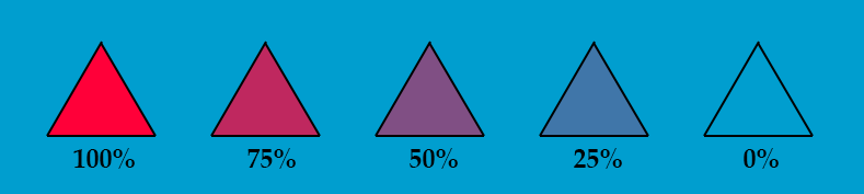
This way the transparency is fully independent of the color values. For example we can have fully transparent color that is either red or blue. One of the main problem with this is that if we sample the texture by floating point precision (for example by using bi-linear filtering) we could encounter color bleeding issue shown in this video.

If we decrease the value of alpha, then the current color is taken less into account when blending.

Premultiplied Alpha

Another way to think about transparency is:

• RGB specifies how much color the objects contribute to the scene
• Alpha specifies how much it obscures whatever is behind it

In math the corresponding equation is:

$blend(source,\; destination) = (source \cdot 1) + (destination \cdot (1 - source_{alpha}))$

Now the RGB and alpha values are linked together. For example the only way to represent full transparency is to set both RGB and alpha channels to zero. In order to convert straight alpha color into the premultiplied alpha color we have to multiply the RBG values with the alpha value.

$premulitpliedAlphaColor = (R \cdot A, G \cdot A, B \cdot A, A)$

Advantages of using premultiplied alpha:

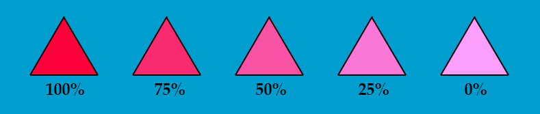
1. No bleeding issues. With bilinear filtering the result with mixed color and alpha values is incorrect, because all fully transparent pixels also have an arbitrary color assigned to them. If we use conventional alpha blending the arbitrary color is also blended to the result. The example on the right illustrates that. The color of the fully transparent pixels is white. With premultiplied alpha blending the only possibility is black and the interpolated values will be correct.
2. The blend function has one less multiplication, therefore it is slightly faster (the multiplication has already been done when the image was saved)
3. Both normal and additive blending can be done with one step without breaking the batching
4. By decreasing only the alpha value we can transform smoothly from normal to additive blending which allows some cool effects for example fire transforming into smoke.

NB! Usually the information whether an image straight or PMA is not stored in the image file itself and it has to be made sure by ourselves. If we mix those two things together (for example export image as premultiplied alpha but render it as straight alpha) we would get strange artifacts like thick black border around the image.

If we decrease the value of alpha here, the current color is still taken into account fully, but the background is considered more and more.

Blend Function

If we compare regular and premultiplied alpha math equations they seem to be quite similar. In practice it is more generalized and has following form:

$blend(source,\; destination) = (source \cdot sourceBlendFactor)\; blendFunction\; (dest \cdot destinationBlendFactor)$

Usually there are different parameters we can assign in order to control the sourceBlendFactor, destinationBlendFactor and blendFunction values. In OpenGL, there is a glBlendFunc() method to configure the blending factors, and the glBlendEquation() method to configure the function.

For example, if we want to represent straight alpha blending we can choose following constants: 

• sourceBlendFactor = GL_SRC_ALPHA
• destBlendFactor = GL_ONE_MINUS_SRC_ALPHA
• blendFunction = GL_FUNC_ADD

If our image is in premultiplied alpha format we have to change:

• sourceBlendFactor = GL_ONE

Some Useful Types of Blending Functions (for Straight Alpha)

Additive blending illustration

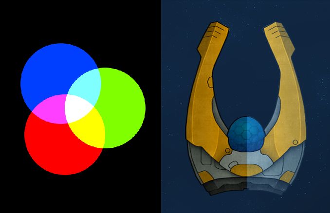
Additive blending

• Behaves similarly to the light
• $blend(source,\; destination) = (source \cdot 1) + (destination \cdot 1)$

Multiplicative blending illustration

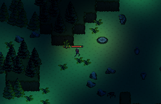
Multiplicative blending

• Useful for creating shadows
• $blend(source,\; destination) = (source \cdot 0) + (destination \cdot source)$

For further experimentation I suggest to try this application: http://www.andersriggelsen.dk/glblendfunc.php