Geometry and Transformations I
We can define a coordinate system and a set of points in it. We saw that depending on the order of those points, we can define many polygons and objects. Larger polygons can be represented as a set of triangles. Those triangles can be defined as just a list of triangles, a triangle strip or a triangle fan.
What if we would want to change the locations of some of the points? For example if some objects we defined are rotating around another point or changing their size?
Imagine that we have defined an approximation of a sphere to represent a bubble. Not all bubbles are of the same size. We would want to reuse our defined geometry for many bubbles with different size.
For simplicity we will see how to change the size of a one 2-dimensional triangle. The same principles apply also to 3-dimensional geometry and more complex shapes. It is just easier to visualize it in 2D.
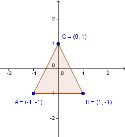
So, we have a triangle with vertices $(-1, -1), (1, -1), (0, 1)$. Notice also that there is kind of a center point (not any of the traditional centers, though) of the triangle at the origin. In order for us to make the triangle bigger, we kind of stretch it with the origin being a fixed point. Because this would be a transformation of our space onto itself (we are not creating any more space and no space is lost), there always will be at least one fixed point. This means that a point $(0, 0)$ would stay the same if we are stretching the triangle.
Okay, so how do we stretch it? If we were to just try and draw a 2 times bigger triangle, we would question that do we want the area to be 2 times larger; or the lengths of the edges 2 times larger; or perhaps we want the coordinate values to represent 2 times larger values.
It happens that it is much easier and uniform to just do the last option. The coordinate value 1 will be 2 times larger, thus 2. Coordinate value -1 will also be 2 times larger, thus -2. Coordinate value 0 will not change.
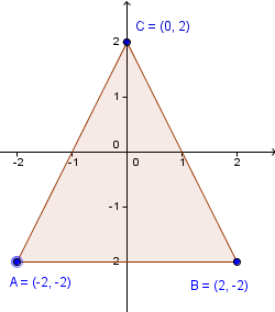
So, we can just multiply all the coordinate values by 2 and get, in some sense, a 2 times bigger triangle.
Here we multiplied both the x and y coordinates of each point with 2. So our algorithm would go through all of the points we have sent to the GPU and do the multiplication of coordinates.
It might happen that sometimes we want to multiply only the x coordinate and keep the y coordinate the same. We might also have different non-unit coefficients for both coordinates. Or it might happen, that we want to add to the x coordinate some multiple of the value of the y coordinate.
This seems like a lot of requirements. Some readers might have already guessed, that a general way to represent those kinds of transformations would be a matrix. Applying the transformation is multiplying the specific point with a concrete matrix.
Our example before would look like this:
$ \left( \begin{array}{cc}
2 & 0 \\
0 & 2
\end{array} \right)
\cdot
\left( \begin{array}{cc}
x \\
y
\end{array} \right) =
\left( \begin{array}{cc}
2x + 0y \\
0x + 2y
\end{array} \right) =
\left( \begin{array}{cc}
2x \\
2y
\end{array} \right)
$
As you can see, when we apply such a matrix to all of the points, we will have transformed our objects. This is the point of the vertex shader in the GPU. It will go through (in parallel) all of the vertices and will apply a number of matrices to them.
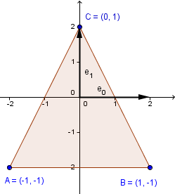
There are other ways to think about transformations. For example you can reach the same shape if you keep the coordinates the same, but think of the basis vectors to be 2 times bigger (represented as $(2, 0)$ and $(0, 2)$ in the original coordinate system).
You might also notice, that this is exactly what we have in the columns of our transformation matrix. So in order to find out, what a transformation does, one can look at the columns of the transformation matrix and see how a new basis would look like.
Here are a couple of definitions:
- Vertex shader – code that is executed in parallel for each of the vertices.
- Transformation matrix – a matrix that holds a specific transformation of the geometry.
- Column major format – convention to hold the space elements (points, vectors) as algebraic column vectors. This allows the multiplication with a transformation matrix from the left.
- Row major format – convention to hold the space elements (points, vectors) as algebraic row vectors. This allows the multiplication with a transposed transformation matrix from the right.
Linear Transformations
There is a notion of linearity with different transformations. As you might remember from previous studies, linearity of a transformation is defined as:
$T(\alpha_0 \cdot u_0 + \alpha_1 \cdot u_1) = \alpha_0 \cdot T(u_0) + \alpha_1 \cdot T(u_1)$,
where $\alpha_0$ and $\alpha_1$ are scalars; $u_0$ and $u_1$ are elements of our space.
This says that the transformation is distributive over addition (additivity) and over scalar multiplication (homogeneity of degree 1).
This is not entirely useful by itself, but it follows that every linear transformation can be represented as a transformation matrix. Also all matrices with fixed scalars in them, define linear transformations. We can also prove the latter with relative ease. Imagine the following:
$ \left( \begin{array}{cc}
a & b \\
c & d
\end{array} \right)
\cdot
\left(\alpha_0
\left( \begin{array}{cc}
x_0 \\
y_0
\end{array} \right) +
\alpha_1
\left( \begin{array}{cc}
x_1 \\
y_1
\end{array} \right)
\right)$
We will continue without assuming linearity of the transformation:
$ \left( \begin{array}{cc}
a & b \\
c & d
\end{array} \right)
\cdot
\left(
\left( \begin{array}{cc}
\alpha_0 x_0 \\
\alpha_0 y_0
\end{array} \right) +
\left( \begin{array}{cc}
\alpha_1 x_1 \\
\alpha_1 y_1
\end{array} \right)
\right) =
\left( \begin{array}{cc}
a & b \\
c & d
\end{array} \right)
\cdot
\left( \begin{array}{cc}
\alpha_0 x_0 + \alpha_1 x_1 \\
\alpha_0 y_0 + \alpha_1 y_1
\end{array} \right) =
\left( \begin{array}{cc}
a (\alpha_0 x_0 + \alpha_1 x_1) + b (\alpha_0 y_0 + \alpha_1 y_1)\\
c (\alpha_0 x_0 + \alpha_1 x_1) + d (\alpha_0 y_0 + \alpha_1 y_1)
\end{array} \right)
$
Now we have applied the transformation and can use the distributive properties of scalar multiplication and addition.
$\left( \begin{array}{cc}
a \alpha_0 x_0 + a \alpha_1 x_1 + b \alpha_0 y_0 + b \alpha_1 y_1\\
c \alpha_0 x_0 + c \alpha_1 x_1 + d \alpha_0 y_0 + d \alpha_1 y_1
\end{array} \right) =
\left( \begin{array}{cc}
\alpha_0 (a x_0 + b y_0) + \alpha_1 (a x_1 + b y_1)\\
\alpha_0 (c x_0 + d y_0) + \alpha_1 (c x_1 + d y_1)
\end{array} \right)
$
We can notice that this result is a vector to vector addition and afterwards we can bring the scalars in front of the vectors:
$\left( \begin{array}{cc}
\alpha_0 (a x_0 + b y_0)\\
\alpha_0 (c x_0 + d y_0)
\end{array} \right) +
\left( \begin{array}{cc}
\alpha_1 (a x_1 + b y_1)\\
\alpha_1 (c x_1 + d y_1)
\end{array} \right) =
\alpha_0 \left( \begin{array}{cc}
a x_0 + b y_0\\
c x_0 + d y_0
\end{array} \right) +
\alpha_1 \left( \begin{array}{cc}
a x_1 + b y_1\\
c x_1 + d y_1
\end{array} \right)
$
The last step is to see that those vectors are the result of other vectors multiplied by a matrix:
$\alpha_0
\left( \begin{array}{cc}
a & b \\
c & d
\end{array} \right) \cdot
\left( \begin{array}{cc}
x_0\\
y_0
\end{array} \right) +
\alpha_1
\left( \begin{array}{cc}
a & b \\
c & d
\end{array} \right) \cdot
\left( \begin{array}{cc}
x_1\\
y_1
\end{array} \right)
$
And this is exactly the linearity of a transformation.
A lot can be represented as a linear transformation. We will see some main examples of them next. Still there are some transformations that we would like to have in computer graphics, but are not linear. We will see later, what exactly those are and how can they be represented.
Scale
We already saw a simple scaling example in the introduction, where we scaled in both x and y directions by 2.
In general a scaling matrix would look like this:
$ \left( \begin{array}{cc}
scaleX & 0 \\
0 & scaleY
\end{array} \right) $
It will be applied as:
$ \left( \begin{array}{cc}
scaleX & 0 \\
0 & scaleY
\end{array} \right)
\left( \begin{array}{cc}
x \\
y
\end{array} \right) =
\left( \begin{array}{cc}
scaleX \cdot x \\
scaleY \cdot y
\end{array} \right)
$
So it will just multiply the x and y coordinates by some scalar value. Notice that if both $scaleX$ and $scaleY$ are 1, we will have an identity matrix and the identity mapping that will not change anything.
You can have scalars in the range $[0, 1)$ in order to shrink your space. Notice that if both $scaleX$ and $scaleY$ are 0, then you will shrink everything to infinitely small and thus lose all the geometry.
If you have negative values as $scaleX$ or $scaleY$, then this matrix will reflect your geometry from the corresponding coordinate axis.
You can try this out in the example on the right, which has a square with vertices $(1, 1), (-1, 1), (-1, -1), (1, -1)$. There is a 4x4 matrix there, but ignore that for now. Your scale values will be on the upper-left 2x2 part of it.
Rotation
Another logical transformation would be the rotation. By rotation we mean rotation around a point or a line. In 3D it is quite clear that rotation would occur around some given line. For example Earth rotates around its rotational axis. In 2D we could think about rotation around the origin or alternatively view 2D as a xy plane in 3D and thus the rotation would be around the z axis.
The basic way of defining a rotation, given a coordinate system, would be around one of its axes. Rotation around an arbitrary line would first rotate that arbitrary line to be aligned with one of the axes; then rotate around that axis and lastly reverse the initial rotation. Another way of defining a rotation around an arbitrary axis would be with the use of quaternions.
Let us try to construct a rotation transformation matrix in 2D around the origin (or the imagined z axis). That can be done by taking an arbitrary rotation, seeing what properties we would want there and deriving the matrix values that would depend on the previous coordinates. However, this brute-force construction would include a number of trigonometric identities and is quite lengthy.
Fortunately, we can reuse the fact that columns of the transformation matrix represent the transformed standard basis vectors. So instead of deriving a rotation of an arbitrary point, we can see how it would affect the standard basis vectors. Initially the standard basis vectors are $e_0 = (1, 0)$ and $e_1 = (0, 1)$. With a rotation around the origin we want to preserve the length of those vectors. Also there should always be a 90-degree angle between them. The following image illustrates that.
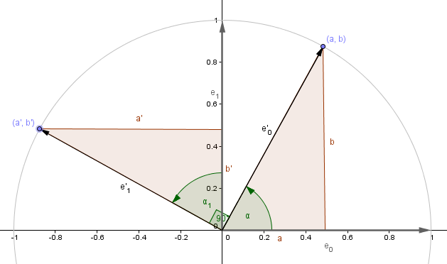
As you can see, the transformed basis vectors would be $(a, b)$ and $(a', b')$. So what values are exactly those $a, b, a', b'$?
We can use the trigonometric function definitions to find them out.
$cos(\alpha) = \frac{a}{|e'_0|} = \frac{a}{1} = a$
$sin(\alpha) = \frac{b}{|e'_0|} = \frac{b}{1} = b$
$cos(\alpha_1) = cos(\alpha) = \frac{b'}{|e'_1|} = b'$
$sin(\alpha_1) = sin(\alpha) = \frac{-a'}{|e'_1|} = -a'$
Because the basis vectors are normalized, their length is 1. Also you can see, that the value $a'$ is represented by a negative $sin(\alpha)$.
So $e'_0 = (cos(\alpha), sin(\alpha))$ and $e'_1 = (-sin(\alpha), cos(\alpha))$.
If we use those values as the columns of the transformation matrix, we will get the rotation transformation matrix:
$ \left( \begin{array}{cc}
\cos(\alpha) & -\sin(\alpha) \\
\sin(\alpha) & \cos(\alpha)
\end{array} \right)
$
And when it is applied:
$ \left( \begin{array}{cc}
\cos(\alpha) & -\sin(\alpha) \\
\sin(\alpha) & \cos(\alpha)
\end{array} \right)
\left( \begin{array}{cc}
x \\
y
\end{array} \right) =
\left( \begin{array}{cc}
\cos(\alpha) \cdot x -\sin(\alpha) \cdot y \\
\sin(\alpha) \cdot x + \cos(\alpha) \cdot y
\end{array} \right)
$
As you can see, here the new values will depend on the values of both of the previous coordinates.
Also the value $\alpha$ should be fixed to some specific angle for linearity. It is not a linear transformation in relation to $\alpha$, only in relation to elements in our space (vectors and points). So it might be more correct to say that a rotation around z-axis by 50-degrees is a linear transformation, not that rotation is a linear transformation.
You can see this matrix in action in the example on the right.
Shear
There is one more linear transformation, that might first seem quite mysterious. We will see later how something quite useful is derived using that transformation. Currently however let us just define the shear with the following matrices:
| Shear x | Shear y |
|---|---|
|
$ \left( \begin{array}{cc} |
$ \left( \begin{array}{cc} 1 & 0 \\ \tan(\phi) & 1 \end{array} \right) $ |
Similar to rotation transformation the value of $\phi$ should be fixed for a specific transform.
Shear transformation kind of tilts one of the axes, this results in moving everything parallel to the other axis in 2D or axes (plane) in 3D. For example, if we use shear-x, then the points are moving parallel to the x axis by $\tan(\phi) \cdot y$. If our $\tan(\phi) = 1$ then the x coordinates of all of the points are shifted by the exact value of their y coordinates. You can test it out in the example on the right.