Volumetric Rendering
When we are rendering, we do not usually think about light interacting with the medium it passes through. We assume light exits from a surface that we see and then reaches our camera, painting the pixel the corresponding color. In most cases, we would be correct to do it that way. The air is transparent, we do not see air. Photons do not interact with air, they just travel through it, right? That works until there is a high concentration of some particles in the air. For examples water particles in clouds and fog, soot particles in smoke and fire, dust particles in an abandoned building. In such cases, the interaction between light and this concentration of particles becomes visible to us. In computer graphics, people call rendering such an effect volumetric rendering, volumetric light transport, volume rendering.
Depending on the situation the density of particles usually varies. The clouds change their shape, fog and smoke are denser in some areas. These areas could even sometimes be moving and making pretty patterns like with flame. Modelling these patterns (changes in the density of particles) is a whole other topic, but for now, we can keep in mind that the density of particles can vary. The simplest approach would be to just map some 3D noise to a location, inside some defined volume of space.
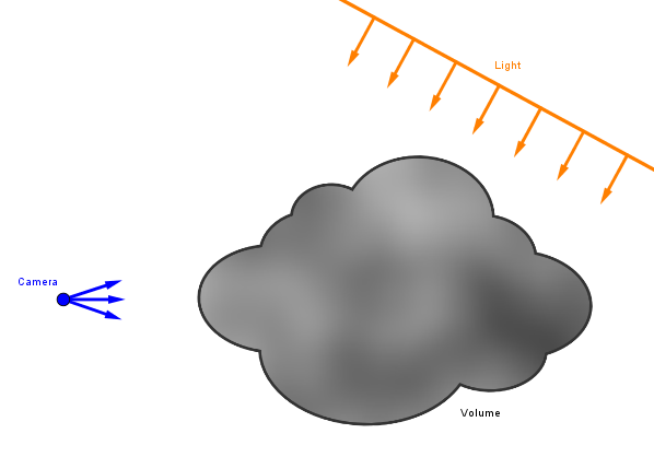
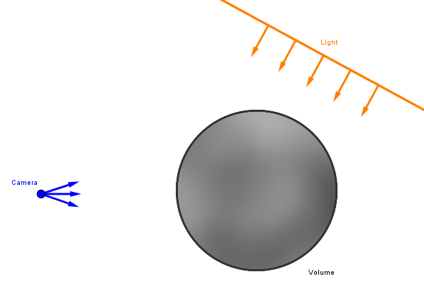
Notice that we have the camera looking that that volume, some light shining on it, and we have something behind that volume too. Although if the volume is dense enough, seeing through it might not be possible. You cannot see a lot through a cloud or dense fog. To keep things simple, in this chapter we will use a sphere as our volume. Depending on the technique, you could have an axis-aligned bounding box surrounding the volume and then a simulated density function (usually still based on noise) inside it. The box can be a good bounding object because volumes like fog, clouds, fire, smoke are usually elongated in some direction.
In this chapter, we are going to look at the optical effects that occur in such volumes and the computer graphics techniques to render them. We will see how the light traverses through this volume, scatters inside it while interacting with the medium, and in the end reaches our camera, coloring a pixel.
Definitions:
- Volume – Somehow defined part of a 3D space.
- (Participating) Medium – Substance that light interacts with when traveling through it.
- Scattering – Light changing direction according to some probability distribution.
- Absorption – The effect of light being absorbed into a substance, dissipating.
- Ray marching – Rendering technique that involves taking sequential samples along a ray.
- Phase function – Function, which tells how much light coming from a certain direction is scattering into another certain direction.
- 3D texture – Texture, which has three spatial dimensions and is thus sampled with three coordinates.
Raymarching and Beer's Law
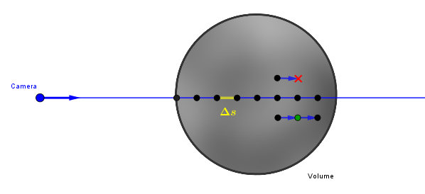
Now, inside this volume, we have a participating medium. The particles of some substance that on occasion interact with the photons traveling through it. Generally speaking, a photon could either pass some particle and continue on its path or not. To simulate this, we will raymarch through the volume and assess the percentage of photons that manage to travel on their straight path across some given length inside the volume. Raymarching in this technique consists of sampling the volume along a view ray some number of times. We march along the ray. These samples could be uniformly spaced or not. In the illustration below $\Delta s$ is our step size for marching the ray. Note that implementation-wise, we just render the volume with the standard pipeline. However, the fragment shader for this volume then proceeds to do the raymarching.
At each sample we can take the length we have marched along the ray and use Beer's law (also known as Beer-Lambert's law) to calculate the percentage of photons that have managed to pass that length through the volume. We call this percentage transmittance. The original Beer's law is quite complicated and more used in chemistry, where the transmittance of a substance can be used to determine what it consists of. In computer graphics we will use a simplified approach:
$\tau(\Delta s) = e^{\Large -\sigma_{extinction} \cdot \Delta s}$,
where:
$\tau$ – The transmittance, giving the percentage of light that was able to pass.
$\sigma_{extinction}$ – Material-specific coefficient, for example, dense clouds have it about 0.03-0.04 m-1. This would be sampled from the volume if it has varying density.
$\Delta s$ – The distance travelled. Note that clouds are several kilometers long, so if we use 0.04 for $\sigma_{extinction}$, our $\Delta s$ should be at least 1000 m.
It is also common to just have a factor of $\sigma_{extinction}$ as a configurable parameter as we might not know it exactly for the effect we make or just want more artistic control. Just make sure your distances are corresponding with that value. Meaning that if you use 0.04 as the maximum extinction coefficient and the distances are in single digits, you will not be seeing any noticeable light absorption.
Code-wise it would be kinda like this:
vec4 raymarch(vec3 samplePosition, vec3 marchDirection, int stepCount, float stepSize) {

    float transmittance = 1.0;

    for (int i = 0; i < stepCount; i++) {
        samplePosition += marchDirection * stepSize;
        transmittance *= exp(-density(samplePosition) * extinctionCoef * stepSize);
        ...
    )

    return vec4(..., transmittance);
}
Here the function density() would be the one generated via noise that specifies the density (or, more specifically, the percentage of extinctionCoef) of the volume at each coordinate. We approximate the density along the length of one step by that single value at each step. We also multiply the individual transmittances together to get the total one. In the end, we will return the total transmittance of light along that view ray path. We could then later use 1.0 - result.transmittance as the alpha value for the given fragment to indicate how much, if not completely, this path through the volume is blocked by the particles.
Transmittance
We have now calculated the transmittance via the Beer's law. It is important to think about how each step in the raymarching contributes to the final illumination. Right now assume that at every step there is some light coming to that location and reflecting back towards our viewer. We will look later at how that light gets there, but for now, every step will have some $light_i$. Our viewer sees a weighted sum of these contributions. At each step we need to weigh the contribution $light_i$ with however much is the transmission of light between that point and the viewer. Thus the weight for step $i$ will be $t_0 ~ \cdot ~ ... ~ \cdot ~ t_i$.
Here is an illustration for that with $i=3$:
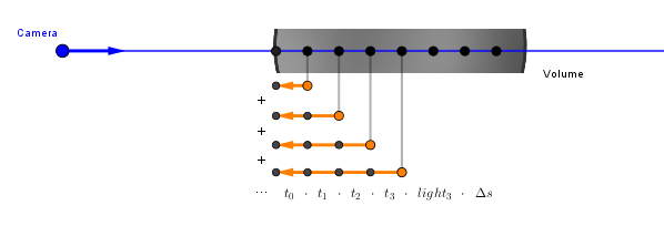
We can read this as just that the final seen light will be however much is transmitted from raymarching step 0, plus however much is transmitted from step 1, plus however much is transmitted from step 2, etc. As in code we already have the current product transmittance calculated, we can just use that as the factor for each contribution. Note that we also have to multiply by $\Delta s$ (stepSize) to normalize the sum. Otherwise, the value would be dependent on the number of steps (would increase if we make more steps).
vec4 raymarch(vec3 samplePosition, vec3 marchDirection, int stepCount, float stepSize) {

    float transmittance = 1.0;
    vec3 illumination = vec3(0.0);

    for (int i = 0; i < stepCount; i++) {
        samplePosition += marchDirection * stepSize;
        transmittance *= exp(-density(samplePosition) * extinctionCoef * stepSize);
        ...
        illumination += transmittance * currentLight * stepSize;
    )

    return vec4(illumination, transmittance);
}
Next, we look at how incoming light reaches these locations, how would we calculate the currentLight value.
In-Scattering
When light is traversing the volume, it is interacting with the particles in it. This causes the light to scatter around in different directions. Imagine driving a car through the fog. When your car's headlights emit light into the fog, the fog becomes illuminated. You can see the light reflecting back from the white fog. An outside viewer may also see the light beams of the car. A similar effect will happen at a concert, where the air is filled with smoke. Often when we sketch a lighthouse or a concert we will draw out these light beams. But the only reason why we see them at all is that some of the light is scattering from the particles in the air and some of that scattered light just happens to be in our direction.
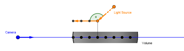
Given one sample point inside the volume, light is coming to it from different directions. Just like when rendering fragments of regular materials, there is actually light coming in from all around the environment. Here we make similar simplifications. We assume that lot of the light is coming in from the direction of some light source (at some angle $\alpha$). It has to pass a portion of the volume to get to our sample point, and that is a separate thing to consider, but that direction can certainly be one source of light. We also assume there is an amount of ambient light bouncing around in the volume. This we can, as with the regular simplest surface lighting models, approximate with a constant.
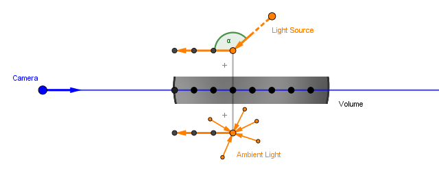
Both of these sources of light we call in-scattering, as the light (wherever it came from) gets scattered towards the viewer. We will come back to the light coming from the light source aspect of this in a bit. For now, we just assume only the simple ambient light contribution.
Out-Scattering
Beer's Law calculates how much of the light transmits through the rest of the volume. However, not all of the light entering our current location is going to travel that way. Some portion of that light gets scattered in a different direction than we assumed. That is called out-scattering, as the light that was traveling towards our viewer, was now scattered out from the view ray.
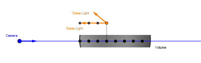
So, our currentLight would be basically inScattering * outScattering. The inScattering would hold the amount of light we get from a light source, ambient scattering in the volume, or some other place (could also be emission, if the particles in the volume are fluorescent). The outScattering will be the percentage of the light that gets redirected from the viewer at the current step. Before we saw the configurable extinction coefficient $\sigma_{extinction}$. This is actually a sum of two coefficients $\sigma_{extinction} = \sigma_{absorption} + \sigma_{scattering}$. The first one specifies how much light is absorbed per unit of volume, the second one indicates the amount scattered. To calculate the outScattering we should use the $\sigma_{scattering}$ part of the coefficient.
Previously we saw that the extinction coefficient would be about 0.04 m-1 for a dense cloud. It varies somewhat, but for clouds, the scattering coefficient part of that would be in the approximate range of 0.01 to 0.06 m-1, and the absorption coefficient would be from 0.000005 to 0.00003 m-1. The absorption coefficient is about three times smaller than the scattering coefficient. Of course, this is for clouds. Depending on the medium, these numbers could be different. So, it could be that these coefficients are grouped together into a single value, or there could be two different configurable values.
uniform vec3 ambientLight;

uniform float absorptionCoef;
uniform float scatteringCoef;

float extinctionCoef = absorptionCoef + scatteringCoef;

vec4 raymarch(vec3 samplePosition, vec3 marchDirection, int stepCount, float stepSize) {

    float transmittance = 1.0;
    vec3 illumination = vec3(0.0);

    for (int i = 0; i < stepCount; i++) {
        samplePosition += marchDirection * stepSize;

        float currentDensity = density(samplePosition);
        transmittance *= exp(-currentDensity * extinctionCoef * stepSize);

        float inScattering = ambientLight;
        float outScattering = scatteringCoef * currentDensity;

        vec3 currentLight = inScattering * outScattering;

        illumination += transmittance * currentLight * stepSize;
    )

    return vec4(illumination, transmittance);
}
Note that we did not do anything complicated here. We just explicitly wrote out the coefficients for absorption and scattering. We also have a variable for the ambient light. Right now we are assuming ambient light is our only source of light. We also refactored our current volume density into a variable and are using it to calculate the out scattering percentage.
On the right is an example of what we have covered so far. There is a Perlin noise function that defines a varying density inside a spherical volume. The density drops off near the borders of the volume. The volume is rotating.
You can modify the ambient light color, which does just that. The parameter V scales the color down (if you want to quickly vary between white and black).
The density slider scales the noise function to zero and allows you to make a thinner volume. The absorption and scattering coefficients are exactly the ones described above. Notice that changing the density, scattering, and absorption coefficients each change the rendering in different ways.
You can also change the number of steps the ray marcher does. It splits the volume into that many evenly spaced samples for each ray/fragment. You can open your Task Manager to see the GPU usage and then turn that slider up to see yourself contributing to global warming. Notice that the render itself does not change noticeably when we change the number of samples. This means that we have normalized our sum correctly.
The Phase Function
Next, we are going to focus on the second part of the in-scattering – the light that comes directly from the light source and scatters toward the viewer at our sample location.
The function that tells us how much of the incoming light scatters towards the viewer is called the phase function. More generally, it specifies how much light scatters towards a direction given some incident vector of light. It is a pretty similar approach to a BRDF function, which would tell us how much light reflects off a given surface in a given direction given some incident light direction. We can approach the phase function in a similar way:
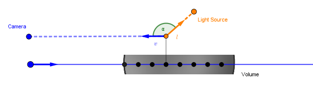
A phase function would be $phase(v, l)$ and would tell us the amount of light that scatters from one of these directions to the other.
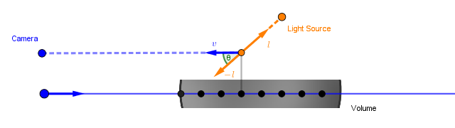
Usually, in phase functions, the angle we are interested in will be the angle between the incident and outgoing vectors. So not the angle $\alpha$ what we would have with regular BRDFs, but rather $\theta = 180^{\circ} - \alpha$. Or, as defined by vectors, $\theta = \angle(-l, v) = \angle(l, -v)$.
There are different phase functions depending on what sort of medium we are modeling. Usually, people talk about Rayleigh scattering, which is the scattering of light in a medium of particles smaller than the wavelength of said light. This is what makes our sky blue and sunsets yellow (because the particles in the atmosphere scatter the blue wavelengths of light through it). Another model of light scattering is Mie scattering. That is a more general approach that also allows the modeling of bigger particles, like droplets of water in the air. The phase functions can get quite complicated. In computer graphics, we usually approach the problem with the Henyey-Greenstein phase function, which was developed in the 1940s when studying light scattering in interstellar dust clouds. So, it models the scattering of light off the bigger (dust-size) particles. The function itself is:
$phase_{HG}(\theta) = \frac{\displaystyle 1}{\displaystyle 4\pi} \cdot \frac{\displaystyle 1 - g^2}{(\displaystyle 1 + g^2 - 2g\cos(\theta))^{3/2}}$
Notice that there is a parameter $g \in (-1, 1)$ here. This determines the isotropy/anisotropy of the function. We will see how this function behaves in a moment. Before, however, people noticed that this function can be quite well approximated by a bit simpler formula (where we do not have to take a root). That easier to compute formula is called the Schlick approximation:
$phase_{Schlick}(\theta) = \frac{\displaystyle 1}{\displaystyle 4\pi} \cdot \frac{\displaystyle 1 - k^2}{\displaystyle (1 - k\cos(\theta))^2}$
On the right, there is an example that visualizes these phase functions in polar coordinates. Given an angle, the distance of the line from the origin depicts the value of the function. Note that as these phase functions need to be energy conservant, their integrals need to sum up to one. This means that if the scattering is isotropic (goes quite equally to all directions), the values of the function will be lower. You can see that is you set the $g$ (or $k$) to $0$. The result is a small circle around the origin.
If the parameter $g$ (or $k$) is positive, then there will be more forward-scattering. Notice that in that case, the largest values of the function are near the $0^{\circ}$ angle. This means that at the angle $\theta \approx 0$, more of the light keeps traveling toward the viewer.
On the other hand, if the parameter is negative, then there will be more back-scattering. This means that more of the light travels at around an angle $180^{\circ}$, the values of the function will be larger there.
Code-wise, we are just going to implement one of these formulae and use it to add a direct light contribution to the currentLight.
uniform vec3 ambientLight;

uniform float absorptionCoef;
uniform float scatteringCoef;

float extinctionCoef = absorptionCoef + scatteringCoef;

vec4 raymarch(vec3 samplePosition, vec3 marchDirection, int stepCount, float stepSize) {

    float transmittance = 1.0;
    vec3 illumination = vec3(0.0);

    for (int i = 0; i < stepCount; i++) {
        samplePosition += marchDirection * stepSize;

        float currentDensity = density(samplePosition);
        transmittance *= exp(-currentDensity * extinctionCoef * stepSize);

        float inScattering = ambientLight + directLight * phase(v, -l);
        float outScattering = scatteringCoef * currentDensity;

        vec3 currentLight = inScattering * outScattering;

        illumination += transmittance * currentLight * stepSize;
    )

    return vec4(illumination, transmittance);
}
Note that both of our $v$ and $l$ are in local space, then v = -marchDirection. Of course, they could also be in camera space, like with regular lighting calculations. Whatever the choice, they both need to be in the same space. To get the cosine of $\theta$ we make sure our direction vectors are normalized and use the dot product.
One last piece of the puzzle here is the directLight amount. That needs to be the amount of light that reaches our current sample through the rest of the volume towards the light source.
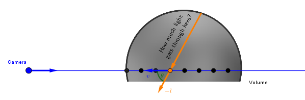
One way to assess this would be to do another raymarch from our current sample towards the light direction until the end of the volume. During that, we could calculate Beer's Law again and thus get the transmittance of the path to the light. With modern computers that is entirely possible to do. However, here we next propose an alternative approach.
Opacity Shadow Maps
We can use a technique similar to shadow mapping to peer into our volume from the light's perspective. With regular shadow mapping, we only get the distance to the closest point of any opaque object. There exist several techniques that are able to record the transparency (transmittance) along different depths from the light. With such extended maps, we could then ask how much light is reaching through the scene to a point at some given distance (depth) from the light. Examples of such techniques are Opacity Shadow Maps, Deep Shadow Maps, and Transmittance Function Maps. Opacity shadow maps are in some sense the most intuitive, so we are going to use these here.
As regular shadow mapping, we start with rendering the scene from our light source. With directional light sources, we use an orthographic camera, with point light sources, we use a perspective camera. Right now we continue with a directional light source. We do not render just the closest value, rather we ray march with even steps of $\Delta z$ some encapsulating volume from a defined $z_{min}$ to $z_{max}$. So, we will record for each pixel several transmittance values at different depths. We could call these layers.
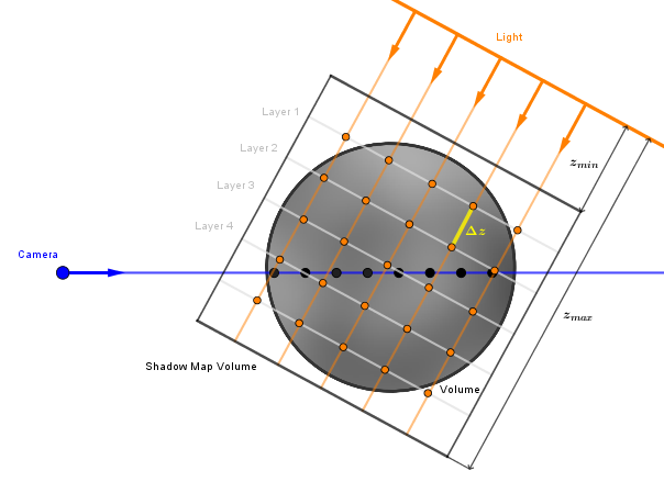
In the most basic solution, rendering every layer would need a separate pass. However, we can use the multiple render targets (MRT) feature to write several values at once. Although, the number of render targets with MRT is limited. The minimum count is 8. This still means that with the minimum of 8, if we want 16 samples, then we can just do 2 (and not 16) passes. One might think that we could also store values from different layers to the different color channels. For example, the transmittance at Layer 1 would go to the red channel, the transmittance at Layer 2 would go to the green channel, etc. That is one way to store four times more values per pass, but it has a problem that becomes obvious later when trying to read the values.
To pass the opacity shadow map to the main rendering pass, the logical choice is to use a 3D texture. All the values are neighbors in the x, y, and z directions. Because we want to avoid aliasing, we can use bilinear (or is it trilinear for a 3D texture?) interpolation. That way we can sample the 3D texture at the coordinate of our main rendering pass ray march sample and get a smoothly interpolated value. But this only works if we limited ourselves to rendering only to one channel before. If we stored different values in the red, green, blue, and alpha channels, the built-in interpolation cannot sample and mix the results correctly. Unless we restructure our data every frame, which would be quite expensive.
Implementation-wise there are a few more things to consider. For example, when rendering from the light camera, we render only our participating media volume, which in our example is the sphere. All the rest of the pixels in the opacity shadow map will have full transmittance. The opaque objects, which can also shadow the volume, could be detected via a regular shadow map pass.
There may still be visible banding because of the low number of layers in the opacity shadow map. In that case, one option is to have a small random offset in each step of the ray marcher. This may create some visual noise instead of banding, but that could then be gotten rid of by a blur if it is too noticeable.
Calculating the transmittance values in the opacity shadow map will be pretty similar to how we calculated the transmittance before. The shader code could be like this:
layout(location = 0) out vec4 outColor0;
layout(location = 1) out vec4 outColor1;
layout(location = 2) out vec4 outColor2;
layout(location = 3) out vec4 outColor3;
layout(location = 4) out vec4 outColor4;
layout(location = 5) out vec4 outColor5;
layout(location = 6) out vec4 outColor6;
layout(location = 7) out vec4 outColor7;

...

// When we render the current fragment, we want to start the march always from the plane at z_min.
// Source: https://stackoverflow.com/questions/9605556/how-to-project-a-point-onto-a-plane-in-3d
vec3 projectPointToPlane(vec3 point, vec3 planeOrigin, vec3 planeNormal) {
    vec3 v = point - planeOrigin;
    float distance = dot(v, planeNormal);

    return point - distance * planeNormal;
}

const int sliceCount = 8;

void main() {

    vec3 position = projectPointToPlane(
        interpolatedPosition,
        vec3(0.0, 0.0, -shadowVolumeRange.x), // Origin of the plane in camera space
        vec3(0.0, 0.0, -1.0) // Camera plane normal in camera space
    );

    vec3 localPosition = (inverse(modelViewMatrix) * vec4(position, 1.0)).xyz;
    float stepSize = (shadowVolumeRange.y - shadowVolumeRange.x) / float(sliceCount);

    float layer[8] = float[](0.0, 0.0, 0.0, 0.0, 0.0, 0.0, 0.0, 0.0);

    float kmToM = 1000.0;
    float extinctionCoef = (absorptionCoef + scatteringCoef) * kmToM; // 0.04 is average coef for dense clouds, 1 unit = 1km
    float currentDensity = 0.0;
    float totalDesnity = 0.0;

    for (int i = 0; i < sliceCount; i++) {

        currentDensity = density(localPosition - float(i) * l * stepSize);
        totalDesnity += currentDensity;

        layer[i] = exp(-totalDesnity * stepSize * extinctionCoef); // Use the Beer's Law to calculate the transmittance and store it

    }

    outColor0 = vec4(layer[0]);
    outColor1 = vec4(layer[1]);
    outColor2 = vec4(layer[2]);
    outColor3 = vec4(layer[3]);
    outColor4 = vec4(layer[4]);
    outColor5 = vec4(layer[5]);
    outColor6 = vec4(layer[6]);
    outColor7 = vec4(layer[7]);
}
In the main rendering code, we transform our current coordinate to the shadow map space and sample the 3D texture:
uniform vec3 ambientLight;

uniform float absorptionCoef;
uniform float scatteringCoef;

uniform mat4 modelMatrix;
uniform mat4 lightCamMatrix;
uniform vec2 shadowVolumeRange;
uniform sampler3D opacityShadowMap;

float extinctionCoef = absorptionCoef + scatteringCoef;

float sampleInScattering(vec3 samplePosition) {
    vec3 shadowMapPosition = (lightCamMatrix * modelMatrix * vec4(samplePosition, 1.0)).xyz;
    float z = (-shadowMapPosition.z - shadowVolumeRange.x) / (shadowVolumeRange.y - shadowVolumeRange.x);
    vec2 uv = shadowMapPosition.xy / lightCamSize / 2.0 + vec2(0.5);

    return texture(opacityShadowMap, vec3(uv, z)).r;
}

vec4 raymarch(vec3 samplePosition, vec3 marchDirection, int stepCount, float stepSize) {

    float transmittance = 1.0;
    vec3 illumination = vec3(0.0);

    for (int i = 0; i < stepCount; i++) {
        samplePosition += marchDirection * stepSize;

        float currentDensity = density(samplePosition);
        transmittance *= exp(-currentDensity * extinctionCoef * stepSize);

        float inScattering = ambientLight + directLight * phase(v, -l) * sampleInScattering(samplePosition);
        float outScattering = scatteringCoef * currentDensity;

        vec3 currentLight = inScattering * outScattering;

        illumination += transmittance * currentLight * stepSize;
    )

    return vec4(illumination, transmittance);
}
On the right, there is a running example of this. You can change the volume's overall density and the absorption and scattering coefficients, just like before with the ambient light example. For the phase function, we use Schlick's approximation, so you can also change its anisotropy parameter $k = k_{Schlick}$. To see the direct light illuminating the volume, you can turn down the ambient light's intensity, which is just a factor for the ambient light term.
The direct light comes from a directional light source, the direction of which is controlled by the azimuth angle $\alpha$ and the elevation angle $\beta$. The $0$ degree for both is to the center-right of the volume as seen from the current view. When increasing the azimuth angle $\alpha$, the light moves around the y-axis in counter-clockwise order. Thus $\alpha = 90^{\circ}$ and $\beta = 0^{\circ}$ would shine the light from exactly behind the volume. The elevation angle $\beta$ increases counter-clockwise around -z (so counter-clockwise as seen from our view). Thus $\alpha = 0^{\circ}$ and $\beta = 90^{\circ}$ would shine the light from exactly the top of the volume.
The shadow map volume parameters $z_{min}$ and $z_{max}$ change the area inside which the shadow map is sliced. If the $z_{min}$ is too big, it may already start inside the volume, thus making the side of the volume facing the light incorrectly too dark. As there are only 8 samples, we want to optimize the shadow map volume such that it covers the volume efficiently.
The last parameter just adds a random jitter to the step size of the volume rendering's ray marches. If there are visible bands, this can help hide them with the cost of adding noise.
The buttons on top of the controls allow you to switch the view between the rendering and the seeing slices of the opacity shadow map. The volume is also rotating, which can be turned off. The rightmost [●] button adds a fixed high-density spot to the volume. If that spot is enabled and it is between the volume and the light source, one could view the shadow it casts through the volume.
Feel free to experiment.
There are several more improvements and similar techniques devised to this. One more example would be the Deep Opacity Map, which starts taking the ray march samples only from the volume's surface. This requires fewer layers to get comparable results, but because the samples are no longer in a spatially uniform grid, we cannot use a 3D texture for storing and interpolating them.
Links
- Real-Time Volumetric Rendering (2013) – Benoit Mayaux
Course notes that neatly cover almost all we covered here. - Volume Rendering for Developers: Foundations – Scratchapixel
Easy to understand and thorough material about what we also covered here. - Volumetric Lighting for Many Lights in Lords of the Fallen (2014) – Benjamin Glatzel
Slides from a graphics programmer's presentation. - Physically-Based Rendering: 11. Volume Scattering (2018) – Matt Pharr et al
This chapter in the PBR book talks about the scattering effects, phase functions, and different mediums. - Physically-Based Rendering: 15 Light Transport II: Volume Rendering (2018) – Matt Pharr et al
This later chapter goes into more mathematics of light transport through a medium. - Physically Based Sky, Atmosphere and Cloud Rendering in Frostbite (2016) – Sébastien Hillaire
How they do it in the Frostbite engine. - Volume and Participating Media (2009) – Yung-Yu Chuang
Slides about volume rendering. - Volumetric Fog Rendering (2019) – Siim Raudsepp
Bachelor's thesis about the volumetric rendering of fog. - Volumetric Clouds Rendering (2019) – Jaagup Kuhi
Bachelor's thesis in Estonian about the volumetric rendering of clouds. - Volumetric Atmospheric Effects Rendering (2018) – Dean Babić
Another thorough Bachelor's thesis about the volumetric rendering of clouds, this time in English. - Volumetric Clouds (2019) – Abhishek Arora
Implementation of volumetric clouds in a custom rendering engine with GitHub code references. - Creating a Volumetric Ray Marcher (2016) – Ryan Brucks
Another implementation, this one is with Unreal Engine. - Real-Time Volumetric Shadows (2011) – Alexandru–Teodor Voicu
A project and a Master's thesis about opacity shadow maps and other similar techniques. - Monte Carlo Methods for Volumetric Light Transport Simulation (2018) – Jan Novák et al
A very involved paper about different volume rendering techniques. - Assessment of cloud optical parameters in the solar region: Retrievals from airborne measurements of scattering phase functions (2019) – Olivier Jourdan et al
Table 2 lists some extinction coefficients measured in clouds.