Deferred Rendering
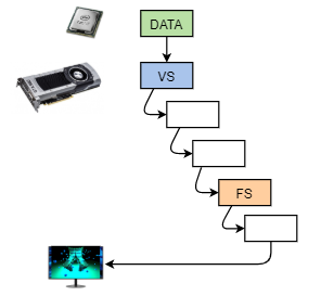
The standard graphics pipeline way we learned to render in the Computer Graphics course was called forward rendering. The GPU is built for doing that. We sent the data and commands into the pipeline and got the result out.
However, forward rendering does have some issues. Notably as the depth test is the last step in the pipeline, lot of the shaded fragments may get overwritten. When we have a complicated fragment shader, it will result in wasted performance. Furthermore, if we have many light sources, then in the shader we would have a loop over all of them. The contributions from each light source would be calculated and added together, even if they are very small (ie the light source is actually far away).
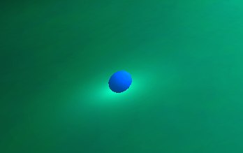
The example on the right includes such a scene. There are 120 point light sources moving around and the fragment shader loops over all of them. You can tweak the attenuation parameters to see that often the point light sources have quite a limited area of effect. Depending on your GPU the example could be quite slow. The example includes stats, so you can also check the milli- or microseconds it takes to render one frame and update the scene. Clicking on the stats will switch between different views. Viewing the example in fullscreen with the render mode will be more costly as the number of rendered pixels will be greater.
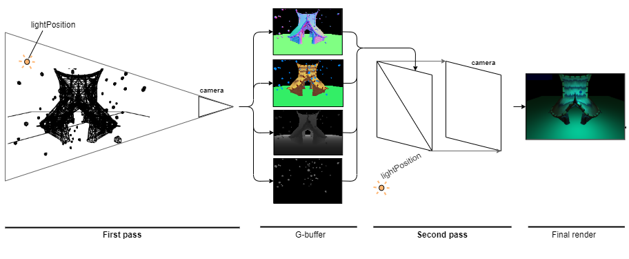
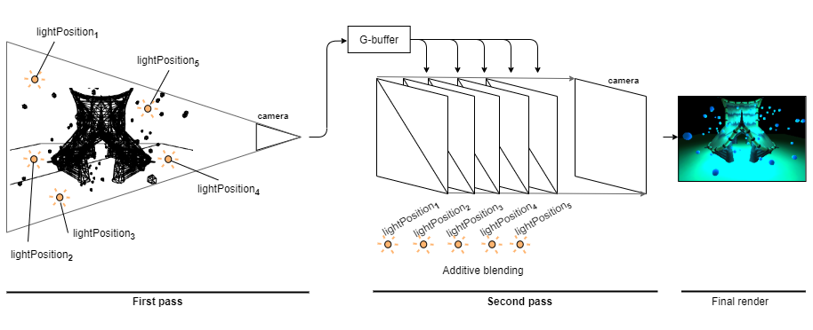
Deferred rendering (also called deferred shading) can solve these issues. The main idea behind it is that we do 2 passes and we do not shade our fragments in the first one. Instead we only write out to a intermediary render target all the values (eg normal, color, depth) necessary for the second pass to shade the fragments. This way the first pass will overwrite the fragments that fail the depth test without too much wasted resources. In the second pass we use the results from the first one to shade only the visible pixels.

While the core idea is easy to understand, there are several things to consider. Like how to get the position from depth, can we optimize it to render areas only affected by the light etc. Deferred rendering has its own pros and cons compared to forward rendering. Depending on the scene or application you are making, one could be more suitable than the other.
Definitions:
- Forward rendering – The traditional rendering flow, where the render (excluding post-processing) is produced by the standard graphics pipeline.
- Deferred rendering – The rendering flow, where one pass of the standard graphics pipeline stores into render targets the data required to shade visible objects. Another pass of the pipeline then combines the data and shades the fragments to produce the render.
- Attenuation – Property of (usually point and spot) light sources that multiplies the light intensity by $1 ~/~ (k_{constant} + k_{linear} \cdot d + k_{quadratic} \cdot d^2)$, where $d$ is the distance to the light source and $k$ values can be configured.
- Stencil buffer – Buffer in the framebuffer, which is written to and used by the stencil test.
- Stencil test – Functionality of the standard graphics pipeline. Values for each pixel can be written to the stencil buffer based on the existing stencil values and fragments passing or failing the depth test. Stencil test can then allow fragments to be discarded based on the stored stencil.
- G-buffer – Collection of render targets that the first pass of the deferred rendering writes to and the second pass uses. Depending on the implementation, the number and nature of the render targets can vary.
- Multiple render targets (MRT) – Technology in WebGL 2 and other newer API-s, which allows one pass to write to multiple different render target textures. This allows the G-buffer to be filled in one pass, otherwise each render target texture would need a separate pass.
- Light volume – Volume that approximates the bounds in which the light source meaningfully contributes to surface illumination.
G-Buffer
The integral part of deferred rendering is the G-buffer. This is where all the data necessary for shading a fragment must be stored. We also want to make it as small as possible as not to waste too much GPU memory. Note that the G-buffer is not copied to the CPU side.
Look back at some of the simplest lighting models. For shading a fragment, the minimum needed input is the material's color, surface normal and fragment position. For example take the Lambert's diffuse model $color \cdot \max(0, n \cdot l)$. We explicitly have the color and surface normal there. We can write the color to the G-buffer target as it is because its values range from $[0, 1]$. We can store the normal vectors by adding $1$ and multiplying by $0.5$, which maps the range $[-1, 1] \rightarrow [0, 1]$.
 |
 |
To find $l$ we need $l = normalize(lightPosition - fragmentPosition)$. We send the $lightPosition$ into the second pass as a uniform. To get the $fragmentPosition$, we have 2 options: 1) Store the position in one of the targets, 2) Store the linear depth and calculate the position from it later.
With option 1) our problem is that we will need a 3-channel buffer, where each channel is either 16 (half-float) or 32 (float) bits. This would result in okay storage of our coordinates. However, it would use at least either $16 \cdot 3 = 48$ or $32 \cdot 3 =96$ bits of memory per pixel. Instead, we can use option 2) and store a depth value of the fragment. It depends on your implementation if you are using the actual depth value (which you could also sample from the depth buffer instead) or have stored the axis distance from the camera (the $-z$ coordinate) either normalized into the frustum or not. If you use too few bits to store the depth, then later on, you can get banding in the values and subsequently in the color calculations:
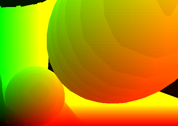 Banding in the position.
|
 Banding in the render.
|
 No banding in the render.
|
In our example we have stored the $-z$ coordinate and normalized it based on the frustum.
 |
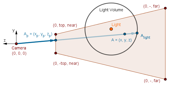
The tricky question, then, is how do we get back the camera space fragment position from just the depth?
For this, we have to remember how we projected camera space points to the near plane in the Computer Graphics course. We were finding the projected coordinates $x_p$ and $y_p$ given some $x$ and $y$.
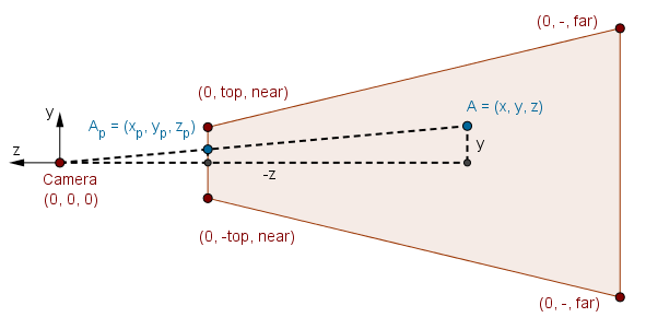
Using similar triangles we found the answers to be $x_p = \frac{x \cdot near}{-z}$ and $y_p = \frac{y \cdot near}{-z}$.
Now, for our second deferred rendering pass we use a quad and an orthographic camera to go through all the screen pixels. We can position that quad to correspond exactly with the near plane. This means that the quad corners would be $(-top, left)$ and $(top, -left)$.
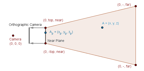
When we are rendering one pixel, the fragment's $x$ and $y$ coordinates will now correspond to the projected coordinates of our point $A$. To find the scene camera space coordinates of $A$ we just do the same derivation with similar triangles as before (or just reverse the previously derived formulae). Resulting in: $x = \frac{-x_p \cdot z}{near}$ and $y = \frac{-y_p \cdot z}{near}$. One has to be careful with the sign here. Depending on which way you have stored the depth value in the G-buffer, the sign of $z$ might be different. In our case, it is actually just $z$, not $-z$ as derived, as we have incorporated the negation into the depth values (so higher values would be further away).
So to get the position from depth, given an orthographic rendering of a near plane quad and the $z$ coordinate derived from the G-buffer value, the formula is just:
$$A = \left( \frac{-x_p \cdot z}{near}, \frac{-y_p \cdot z}{near}, z \right).$$
This now covers all the data that is minimally necessary. However, you might be now thinking what about the alpha channel? The color and normal both take 3 channels, but we can have a 4 channel texture too. Also, in the illustration, we had 4 render targets. Basically, this all comes down to the specific implementation. Naturally, we will need more values per fragment for different lighting models. Phong, for example, would need the specular color (or at least the intensity) and the shininess values.
Right now, we have just used another render target to store, for example, the emission value in one channel. Later we will store the emission in red and specular intensity in green.
 |
Generally, yes, it is up to you to optimize your values and buffers such that you do not waste too much GPU memory.
The example on the right shows the illustrated 4 render targets and their values. The render targets are sampled 1/4th of the size to fit them all on the screen. In reality they are the same size as the viewport.
Links
- Learn OpenGL chapter on Deferred Rendering
Overview of Deferred Rendering - Creating the G-Buffer (2008) – Catalin Zima-Zegreanu
Considerations about what size to use for different values. - Deferred Shading Method in DirectX9 (2019) – DreamAndDead
Thorough overview of Deferred Rendering from light attenuation theory to positioning the near plane quad. - Deferred Rendering: Making Games More Life-Like (2020) – Copperpod
Another overview with real game examples.
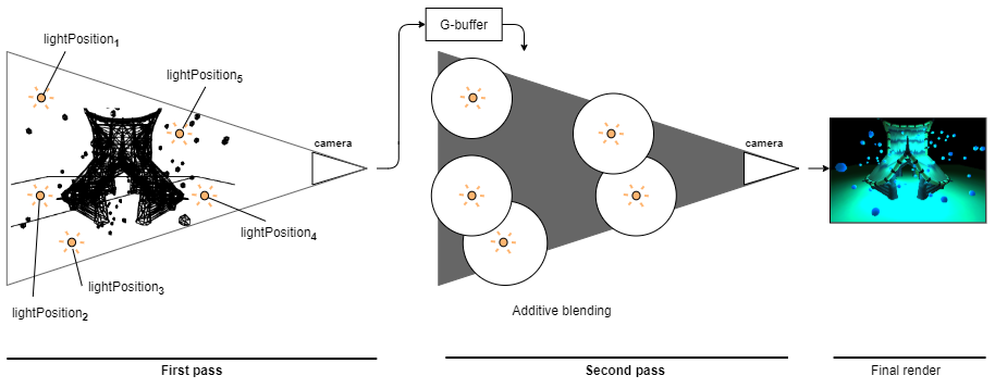
Deferred Lighting
The main benefit of deferred rendering is a performant rendering of many light sources. To render such, we can have a quad for each light source. These quads are rendered in one pass, and the values are blended together additively. This simulates the addition of different light source contributions that we would code in a forward rendering fragment shader. When we want to add ambient light, then we add another quad with a material that adds a small constant contribution.
There are derivations of this as well. For example, only the light contributions could be additively blended, and then we would have a third pass, which would multiply the sum with the material's color. This would be necessary to add gamma correction as well. Because we need to add the different lights/colors together in the linear space and only after the sum moves to gamma space for the monitor. Doing it inside the sum is incorrect as generally: $(a + b)^c \neq a^c + b^c$.
Right now, however, we have only gained performance from the overdraw. This means that while we shade only the visible pixels (not all front-facing pixels as with forward rendering), we are still trying to account for all the lights for all the pixels. Even if we have pixels that are not illuminated by any light source (attenuation will be near 0), we still try to calculate the shading. The next step in optimizing deferred rendering is to use light volumes instead of quads. These are volumes in which the attenuation will not be too small, ie in which there is a meaningful contribution of light.
 Additive blending of lights.
|
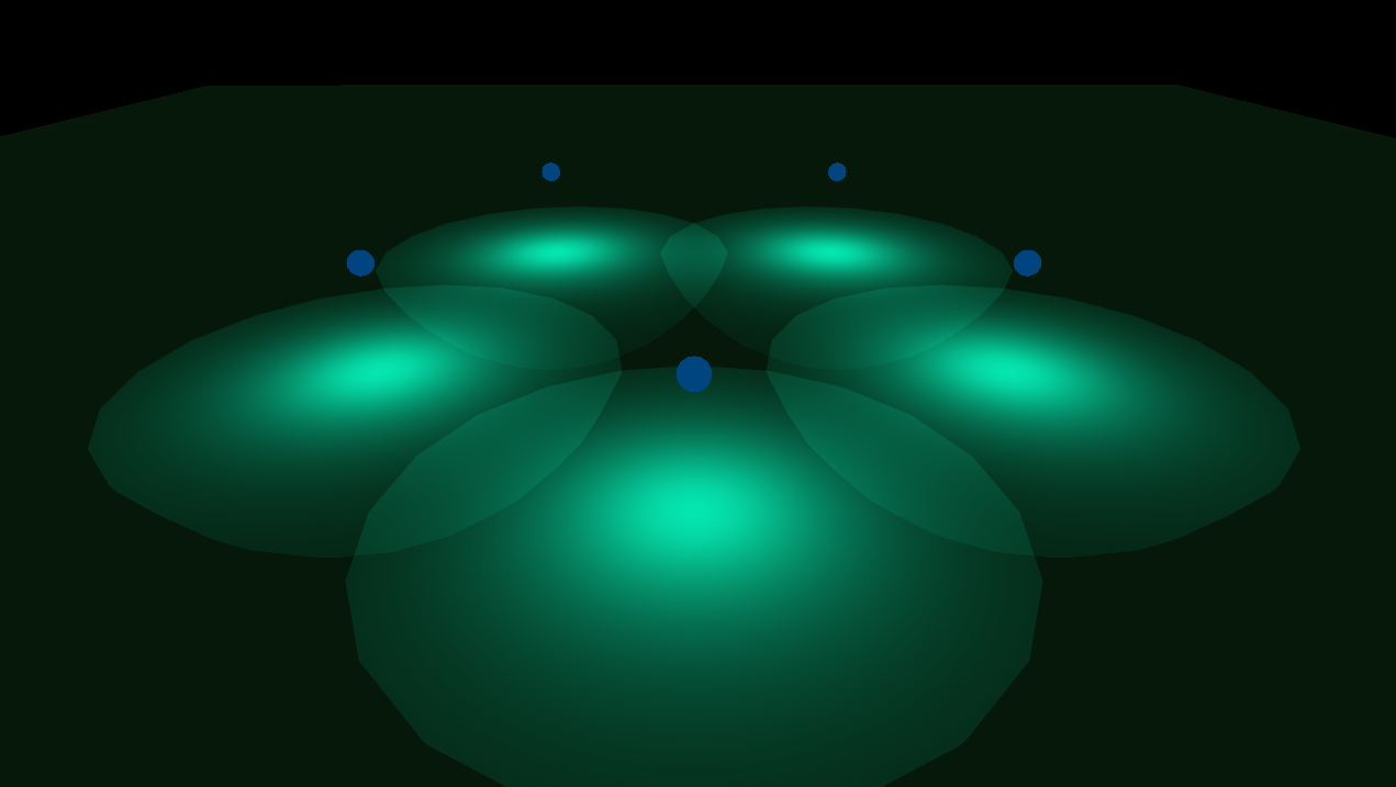
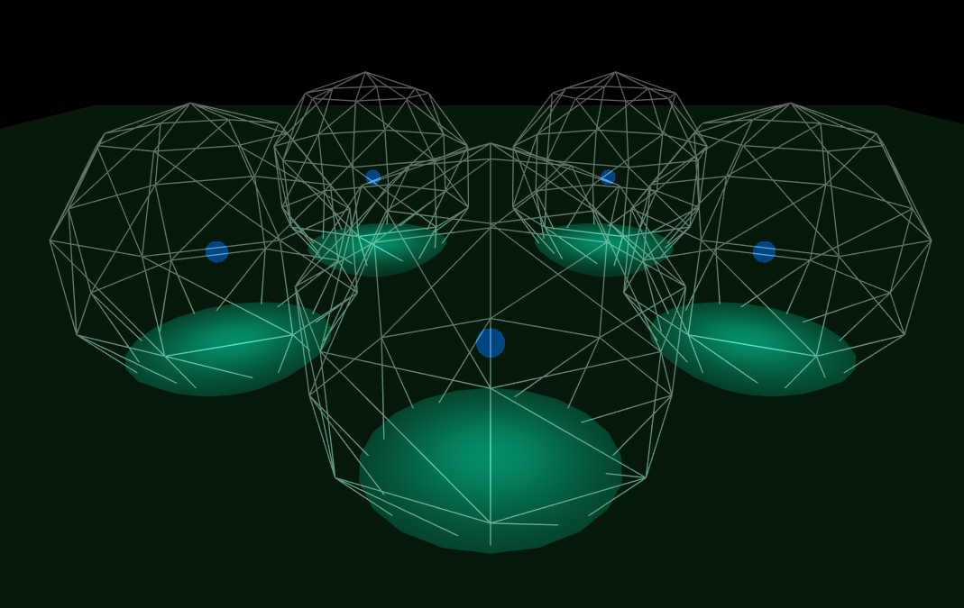 Light volumes.
|
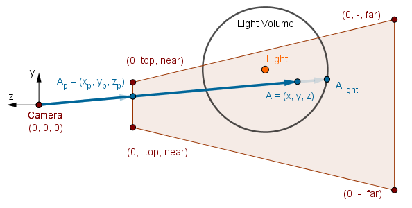
To render the result, we can now use a perspective camera and render a scene of light volumes.
Because we are using a perspective camera, we do not need to worry about placing a quad exactly at the near plane. However, we do have to transform the rendered coordinates to it. When we are rendering a light volume, we get the coordinates of the light volume fragment. We are using the back face of the light volume to render it, as this is part of an optimization we will do later.
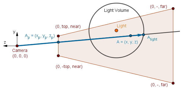
We need to project the light volume fragment's coordinates $A_{light} = (x_l, y_l, z_l)$ to the near plane. This we do the same way as the regular point projection: $x_p = \frac{x_l \cdot near}{-z_l}$, $y_p = \frac{y_l \cdot near}{-z_l}$. This will leave us with a projected point at the near plane, just like we had with the orthographic camera and quads.
The last step is exactly the same as before. We project the near plane coordinate back to camera space, but we use the scene depth from the G-buffer to do it. This will get us to point $A$, which we want to render.
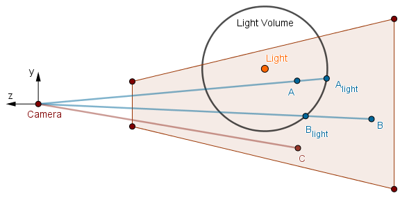
If there are scene fragments that are not on the same path as some fragment of a light volume, then we will not render them. For example, the point $C$ below does not get light calculated for it. However, we have not eliminated all the fragments outside the light volumes yet. In the image below, our algorithm will also try to render point $B$ as it is on the same path as a light volume. Yet it is outside the light volume, and the attenuation will be near 0, so the point will not have a meaningful light contribution. This will be a waste of calculation.
To get rid of cases like the point $B$, we have to approach this one light source at a time. We will use a stencil culling optimization. Consider the following scene:
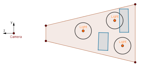
It is evident that only a small section on the top-right is actually illuminated in the scene. The light volume on the left does not contain any scene geometry. The light volume on the bottom-right does not contain any either, but, more importantly, it is occluded by the scene geometry. So even if it would illuminate something, the viewer would not see it.
To detect and handle these cases, we have to render each light source separately and use a stencil test. It turns out that we will need 2 passes per light source. Thus the number of passes after the G-buffer pass would be $2 \cdot numberOfLights$. While this seems expensive, depending on the scene, we can actually win performance from discarding a lot of otherwise unnecessarily shaded fragments. For each light source separately the algorithm works like this:
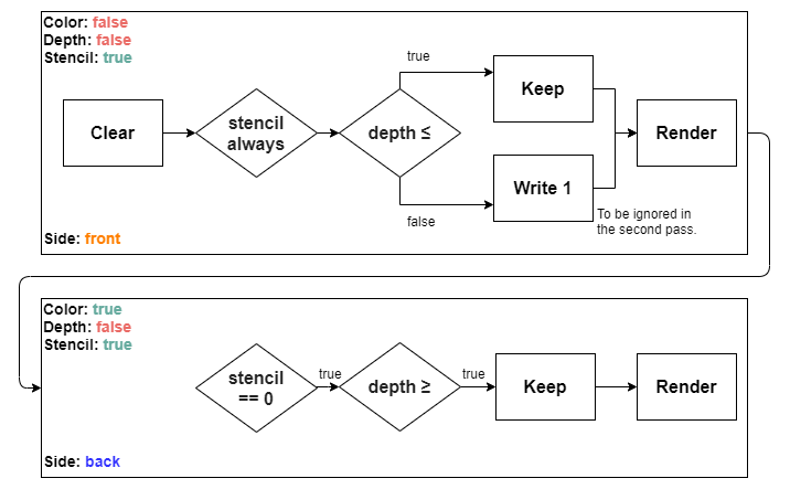
In the first pass here we render the front sides of the current light volume. First step is to clear the stencil buffer to 0. This is to not have other light sources affect the current one. Otherwise we will still render some otherwise ignored fragments if a passing fragment happens to be on the same projection ray. Or it may happen vice versa that we do not render a passing fragment, because a failed fragment is on the same ray. Anyway, we clear only the stencil buffer. We do not clear the color buffer, as that will hold the accumulated final render. We also do not clear the depth buffer, as that holds the scene depth from the previous G-buffer pass.
Then at this pass we let the stencil through, but we check if the depth is less or equal to the scene depth. If it is, we have a potentially visible fragment and we keep the 0 in the stencil. If it is not, then this means that the front side of this volume is behind some scene geometry. Meaning that the scene geometry occludes it and we do not see the fragment or anything behind it in the final render. In that case we write 1 to the stencil buffer.
In the second pass we render the back sides of the current light volume. We also render to the color buffer here, accumulating the final render. Here we use a stencil test to render only the fragments that have 0 in the stencil buffer. If the front face in the previous pass was behind some scene geometry, then everything behind it is too, so we ignore the fragments that got 1 in the previous pass. We then check if the depth here is greater or equal to the scene depth. This means that the back face of the volume is behind some scene geometry. If that is the case, we know that there is scene geometry between the front and back faces of the volume, thus we render that light volume's back face fragment.
You might be wondering that if depth testing is after fragment shading in the pipeline, then will the fragments that fail the depth test in the second pass still get rendered. The answer is usually no, because modern GPU-s actually do an early depth test. There are some conditions for this, but basically it tests the depth before executing the fragment shader. So even though we execute the fragment shader and render to the color buffer, if the depth test fails, the fragment shader is not ran.
Getting back to our example scene, consider the leftmost light volume.
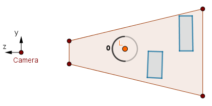 First pass.
|
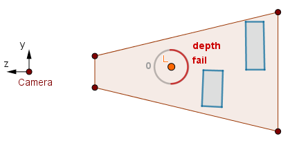 Second pass.
|
In the first pass the fragments pass the ≤ depth test, so we keep the 0 in the stencil buffer. In the second pass the stencil test will pass, but the ≥ depth test will fail as there is no scene geometry before the back faces. Thus we will not render anything to the color buffer.
Consider the top-right volume.
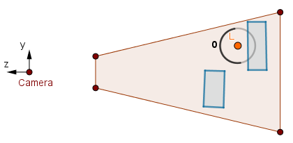 First pass.
|
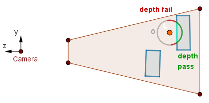 Second pass.
|
In the first pass we keep 0 as before. In the second pass, there are some back faces where the ≥ depth test fails like with our leftmost volume before. But there are also some back faces where there is scene geometry before them, i.e., where the ≥ depth test will pass. These fragments we render and the fragment shader will color in the illuminated scene part.
Consider the bottom-right volume.
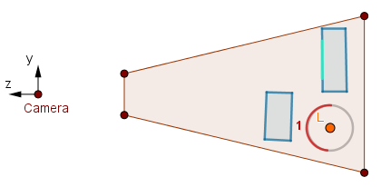 First pass.
|
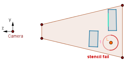 Second pass.
|
In this case the first pass will fail the ≤ depth test as there is scene geometry before the front faces. We write 1 to the stencil buffer. On the second pass, the stencil test will fail as the buffer does not have 0 values. Thus the volume that is occluded by the scene geometry will not be rendered.
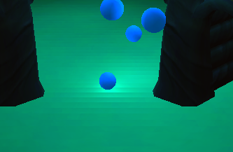
On the right we finally have an example of deferred rendering. It has the same scene and the same 120 light sources as in the forward rendering example we had in the beginning. The Naive Result renders one quad for each light source. The Optimized Result uses light volumes and the stencil culling algorithm just described.
When you look at the Volume Fragments, then each discarded fragment will contribute 10% red. Each passed fragment will set the green and blue to 1, resulting in cyan. If there are discarded fragments on the same ray as a passed fragment, the color will tend to white.
|
|
No fragments on the path | |
|
|
Some discarded fragments. | No passed fragments. |
|
|
At least 10 discarded fragment. | |
|
|
No discarded fragments. | One passed fragment. |
|
|
Some discarded fragments. | |
|
|
At least 10 discarded fragment. | |
The noticeable performance gain depends on your GPU and screen. Because browsers limit the framerate to 60, we can also look at the GPU load. On my computer it happened to be like this:
| Example | Framerate | GPU Load | ||
| Forward Rendering | 48-60 | 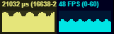 |
87-99% |  |
| Deferred Rendering (Naive) | capped |  |
90% |  |
| Deferred Rendering (Optimized) | capped | |
64-81% |  |
Of course, there exists also other optimizations. Some computer graphics algorithms that, by default, use the forward rendering approach, have their own implementations with deferred rendering. So there are always pros and cons, like the availability and performance of the algorithms we want to use, to consider when choosing between the forward and deferred rendering.
Links
- Position from Depth 3: Back in the Habit (2010) – Matt Pettineo
Explanation on how to get the camera space position given the depth value. - Forward Rendering vs. Deferred Rendering (2013) – Brent Owens
The pros and cons compared. - Rendering deferred lights using Stencil culling algorithm (2009) – Yuriy O'Donnell
The light volume optimization algorithm as originally presented. - Deferred Shading in S.T.A.L.K.E.R. in GPU Gems 2 (2005) – Oles Shishkovtsov
Includes optimizations, shadows, post-effects used together with deferred rendering. - Deferred Shading (2004) – Shawn Hargreaves, Mark Harris (Nvidia)
Presentation about the topic by Nvidia that covers a lot.