Fractal Rendering
Usually, a fractal is described as a visual object with some self-similarity. It is difficult to give a concrete definition because there are many different types of fractals and people may understand the term fractal differently depending on the context. However, we can usually emphasize the self-similarity property of fractals. There is some small-scale part of the fractal that looks like some large-scale part. This could be exactly the same-looking part or could just be similar enough that we see the resemblance. Although that resemblance might be difficult to explicitly point out, we somehow intuitively feel it if something is a fractal.
Fractals can be categorized by different methods that generate them:
- Iterated function systems – These are fractals generated via some geometric rewrite rules. For example, the Koch snowflake is constructed by drawing new triangles in the middle of the outer edges of existing triangles, thus extending the shape. Other commonly known examples are the Sierpiński triangle and the Menger sponge.
- Lindenmayer-systems – As you might have guessed, the L-systems we learned in the Computer Graphics course are also fractals. You can think of a simple tree generated by an L-system. The whole process of iterating the systems inherently creates a fractal structure as the same rules are applied at each iteration to grow the tree. Ie, branches of a tree have a similar structure as the tree itself.
- Strange attractors – Systems of differential equations that evolve in time can create fractal-like shapes.
- Escape-time fractals – These are systems that recursively iterate over the input and try to find if the result stays within some bound (does not escape in some certain number of iterations). The famous Mandelbrot fractal is an escape-time fractal. These will be the fractals whose construction and rendering we will focus on in this topic.
Popular software for fractal rendering includes Mandelbulber, Mandelbulb 3D, Fragmentarium. The best place for everything fractal is Fractalforums (historical site). If you really want to get a retro feel, then you can go to Sprott's Fractal Gallery, where a new fractal is automatically generated every day!
Definitions:
- Fractal – Some kind of object, which exhibits self-similarity at different scales.
- Escape-time fractal – Fractals that arise by iterating a function on some input, usually a complex number, and considering it escaped if its magnitude exceeds some threshold after a fixed iteration count.
- Orbit – Sequence of numbers arising from iterating an escape-time fractal process on a given input (the path this number takes).
- Complex numbers – Number system extending real numbers by adding an imaginary part.
- Imaginary number – The number $i$ such that $i^2 = -1$.
- Dual numbers –Number system extending real numbers by adding an abstract part.
- Abstract number – The number $\epsilon$ such that $\epsilon^2 = 0$ and $\epsilon \neq 0$.
- Distance field – Some mapping $\mathbb{R}^n \Rightarrow \mathbb{R}$, where for any given input the output is the distance to the nearest surface (where the field value is $0$).
- Partial derivative – Derivative showing the change of a multivariate function with respect to a change in one coordinate/axis of the input.
- Gradient – Vector of all the partial derivatives of a multivariate function $\mathbb{R}^n \Rightarrow \mathbb{R}$. Shows the direction of the greatest increase of the function at any given point.
- Jacobian – Matrix of all the partial derivatives of a multivariate function $\mathbb{R}^n \Rightarrow \mathbb{R}^m$. Has the gradients for each output coordinate/axis in its rows.
- Ray marching – Technique to render a distance field by stepping (marching) through it with rays, each the ray length being the value in the distance field at the ray's origin.
- Level surface – Surface that is defined in some specific constant $c$ level, $f(x) = c$. Often $c = 0$.
Julia and Mandelbrot
You probably know quite well how a Mandelbrot fractal sorta looks like. But the Mandelbrot fractal is actually made up of different seeds for Julia sets. It is also called a map or a dictionary of all Julia sets. Julia sets are also a bit simpler than the Mandelbrot, so we will start with these.
Julia Fractal
Julia sets are created from complex numbers. These numbers have 2 dimensions and form a 2D plane, on which we can render the fractal. For each rendered pixel, its coordinate on the complex plane will be the input to a recursive function. As the Julia fractal is an escape-time fractal, we are interested in seeing if the complex number will grow to infinity in that recursive process or not. That recursive function for Julia sets is:
$z_{n+1} = z_n^2 + c$
Here $z_n$ is the result of the process at step $n$. We will start at the pixel coordinate we are rendering. The constant $c$ will be another complex number, which defines a Julia set. Different values for $c$ give different Julia sets.
For example, if we are rendering a pixel at coordinates $(5, 10)$, our initial $z$ will be $z_0 = 5 + 10i$. We also have to define some $c$ and then we iterate the process. If at some point determine that the process grows to infinity, we can color the pixel white. If we determine that it will never grow to infinity, we can color the pixel black and that coordinate will be in the Julia set.
Sometimes will be unclear if the point actually tends towards infinity or not. Commonly a condition is used which checks if the length of the complex number is greater than 2, then we consider it tending to infinity. This produces some false positives into the Julia set, but that is usually okay. When creating fractals we are often interested in the visual look, not that much mathematical accuracy.
Mandelbrot Fractal
If you understand how the Julia fractals are created, then the Mandelbrot fractal is also easy to grasp. The process of the Mandelbrot fractal is the same, but instead of some configurable $c$ we use the pixel coordinate. The pixel coordinate is also the initial $z$ value ($z_0$), so the formula for the Mandelbrot is:
$z_{n+1} = z_n^2 + z_0$
The escape-time condition is usually the same. If the length of $z$ reaches over 2 within some number of iterations, then we exclude the point from the set, else we include it. On the example to the right, you can change the number of iterations and see the shape become more accurate as the iteration count gets larger.
You can also see the different Julia sets and set the complex number $c = a + bi$ to the specific Julia set you wish to check out.
Radial Space Folding
One way to think about how Julia fractals are formed is to see what complex number multiplication does to the space. For that, we should check out our complex numbers in their polar form.
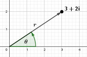
A complex number $z = a + bi$ would be in polar form $z = r \cdot (\cos(\theta) + \sin(\theta)i)$.
When multiplying two complex numbers in polar form, the result has the angles added and radii multiplied together. Generally speaking:
$z_1 \cdot z_2 = r_1 \cdot r_2 \cdot (\cos(\theta_1 + \theta_2) + \sin(\theta_1 + \theta_2)i)$
For Julia sets we are multiplying the complex number with itself, ie, squaring it. Thus:
$z^2 = r^2 \cdot (\cos(2 \cdot \theta) + \sin(2 \cdot \theta)i)$
Generally speaking, we can use any power instead of 2 there.
$z^p = r^p \cdot (\cos(p \cdot \theta) + \sin(p \cdot \theta)i)$
Now we know that the length of the location vector of the complex number (the radius) is raised to the power. If our power is over 1 and the length is also over 1, the length will increase. This means that regardless of the angle when we square complex numbers, the numbers with lengths over 1 will get pushed away from the origin. Similarly, the numbers with lengths less than 1 will get pulled into the origin.
We also now know that the angle will be multiplied by the same power. This means that the complex numbers will sorta rotate on the complex plane. It is not a rotation, though, as numbers with small angles stay more similar than ones with large angles. For example, the square of a number with an angle of 20° will have an angle of 40°, but a square of a number with an angle of 120° will have an angle of 240°. This is illustrated in the image below:
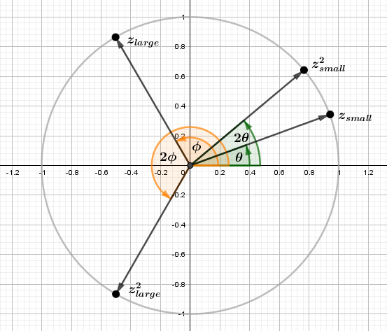
Here the complex numbers are chosen to be of unit length so they would stay on the unit circle. In the Julia fractal, we have a process that keeps raising the numbers to the power 2 many times. We can think about this as a process that in some sense generates more space or, more intuitively perhaps, radially folds the space unto itself. Notice that the same thing happens in the opposite direction with negative angles too.
If this would be all the Julia fractal is doing, we would have a pretty boring fractal – just a unit circle (or a disc, depending on the implementation). The points outside the unit circle would escape quite fast, the points inside would be pulled towards the origin. Luckily, the Julia process also includes an additive term. The constant complex number $c$ added every iteration shifts the space by some amount. This means that some numbers outside the unit circle may end up inside in the next iteration and vice versa. This is what creates the Julia fractal an interesting fractaly look.
We can visualize this space folding in time as is done in the example on right. We are translating the fractal only in the shift step ($+c$). The folding step ($z^2$) kinda centers the fractal back. Try to focus on one spot on the fractal and see how it moves. Note that while in the visualization it seems that space is generated out of nothing, in the actual Julia process the new values come from complex numbers that have gone over 360°.
The red areas in this and the previous example depict the complex numbers for which the process resulted in a complex number with length around 0.5.
There are two other explanations for this: one by Karl Sims and another by Steven Wittens.
Links
- Understanding Julia and Mandelbrot Sets – Karl Sims
Very concise and intuitive explanation - How to Fold a Julia Fractal: A tale of numbers that like to turn (2013) – Steven Wittens
For a mystical experience in understanding complex numbers. - Folding the Julia Fractal (2020) – JP
Different animation options, including an interesting shadertoy. - Julia Set Fractal (2D) (2001) – Paul Bourke
Brief intro into Julia sets with pretty pictures.
Coloring
You have probably seen some really awesomely colored fractals before. It is not immediately obvious how to actually color Julia or Mandelbrot sets. The examples above had binary values – the pixel coordinate either belonged to the set or not. We did draw some stripes to keep track of part of the structure inside the set, but that was about all we did. Furthermore, people often color the outside of the fractal rather than the inside. To use more than just 2 colors for that, we would need more values to map these colors against. One value we do have for the outside points is the escape time of a point. Ie, the number of iterations a point went through before escaping the set. Remember that escaping the set meant that its length became larger than some fixed value. We will call this value the bailout value (B). This is one of the easiest colorings to do, just take the escape time value (iteration count) and map it against some colors. We could normalize it via the maximum iteration count and use it to mix between different colors.
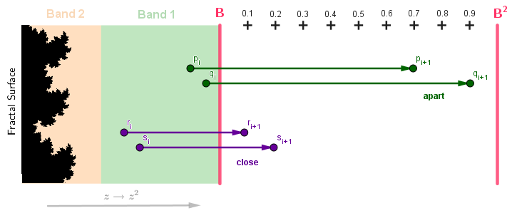
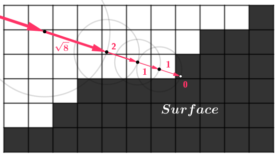
This solution, as you can guess, will create visible banding. Because our escape time values will be integers (1, 2, 3, ...) representing on which iteration our point escaped, the color mix we do, will also have these discrete bands. This could be the desired look, of course, but if we could make a smooth coloring instead, then that would perhaps make the fractal pop out more and thus be aesthetically nicer. It is possible to derive a smooth iteration count and thus make a smooth coloring. To do that, we will consider a single direction from the surface of the fractal. The value B will be our bailout value (after what length do we consider the point to be escaped). We also simplify the case to 2 bands.
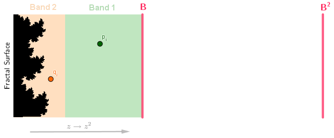
The points in Band 1 need one more iteration to escape. The points in Band 2 will need 2 iterations. We have two example points here too: $q_i$ from Band 1 and $p_i$ from Band 2. The index $i$ shows that these points have already passed through $i$ iterations themselves. They are calculated from some original pixel coordinate points $q_0$ and $p_0$. The chain of $p_0, p_1, p_2, ..., p_i, ..., p_n$ is called an orbit. In this example, when we move forward along an orbit, ie, iterate the Julia function $z_{i+1} = z_i^2 + c$ on a point, the point always moves directly to the right. We will also make a simplification to the Julia function by omitting $+c$. For larger numbers, the $+c$ term becomes unimportant compared to the $z^2$ term. So, when we calculate the next step in the orbits, we just square the lengths.
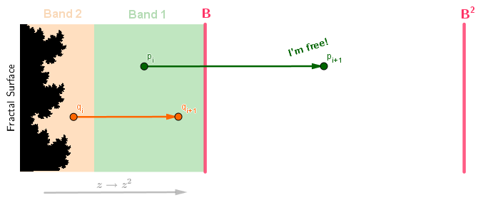
Our point $p$ has now escaped (crossed the length threshold $B$) at escape time $i+1$. So, wherever the point $p$ came from, we will color it the color corresponding to index $i+1$. The second point $q$ has not escaped yet, but obviously will in the next iteration, thus its escape time will be $i+2$ and we will color its origin some other color. If it is the case that $i=0$ and thus $p_i$ and $q_i$ are the origin points in this example, then we will color them and other pixels in Band 1 and Band 2 different colors.
Now we would like to make the coloring smooth. Basically, we would need one value from $[0, 1]$, which tells us how far along in some band our point is. Notice that because we are only squaring our points, their proportional place in every band will be exactly the same. The point $p_i$ was in about the center of Band 1 and will be in the center in the band from $B$ to $B^2$. The point $q_i$ was roughly $2/3$ through Band 2 and $q_{i+1}$ is at the same proportion in Band 1. So, if we can find that smoothly changing value from $[0, 1]$ for one band, we can directly apply it on the origin point and the result should be a smooth coloring over origin points.
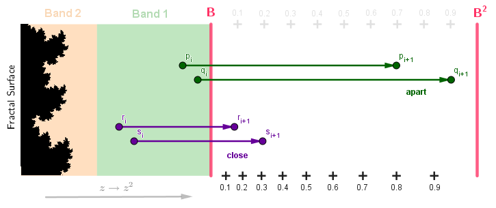
Let us take the band $[B, B^2]$. This is the band where all the escapees will end up first in when escaping. They have to cross $B$ to escape and they will not be crossing $B^2$ in a single iteration. This is because one iteration only squares the number $z^2$. The points near $B$ should get the values from $0$ (because they are at the beginning of a band) and the points near $B^2$ should be getting values near $1$ (as they are reaching the end of the band). Thus we want to map $[B, B^2]$ to $[0, 1]$.
If we just take the proportion of the distance traveled on the escape band, then we would surprisingly not get a smooth coloring. Because our process always squares the numbers. If we start with a uniform pixel grid, then each iteration the numbers with higher initial values will get more spread apart than lower numbers. Our process is not linear, so just a linear range conversion in the escape band based on the distance there will not work out. For example, we can consider two pairs of points in Band 2. Both points in both pairs are close to each other. One pair, $p_i$ and $q_i$, is at the end of the band and another pair, $r_i$ and $s_i$, is at the beginning of the band. Next iteration all the points will escape, but points $p_{i+1}$ and $q_{i+1}$ will be more apart than the points $r_{i+1}$ and $s_{i+1}$.
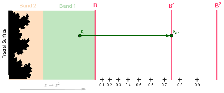
So, instead of splitting the escape band space equally, we rather want to find how much the exponent of $B$ needs to increase from $1$ to be at that distance.
In the picture above you can see that the distance in terms of the exponent increase of $B$ will now be about $1.5$ for both pairs of points.
To find the exponent increase, we can first find the exponent itself via: $\log_B(|p_{i+1}|) = \log(|p_{i+1}|) / \log(B)$
Then we could just subtract $1$ from that to get the $B$ exponent offset. This we subtract from the discrete integer iteration count to get a smooth continuous iteration count. We can then use it to mix between some colors or sample from a continuous color palette.
Unfortunately, we have again jumped the gun a bit. By subtracting $1$ we are doing a linear mapping. Generally that transformation would be $(\log_B(|p_{i+1}|) - 1) / (d - 1)$, where $d$ is the exponent we use to iterate our process (in our case with Julia and Mandelbrot fractals it's just $2$). What we actually found with $\log_B(|p_{i+1}|) = e$ was some exponent $e$ such that $B^e = |p_{i+1}|$. Now, this $B^e = p_{i+1} = {p^2}^{i+1}$, we have raised our point $p$ to the power of $2$ some $i+1$ times for it to escape. If we want to find out what is the offset of the iteration count for $B^e = p_{i+1}$, we need to find the fraction of the iteration we did to get from $B^1$ to $B^e$. Our Julia process was $p^2$ and this also applies to $B$. So, what we actually have is $B = {B^2}^0$ and then some $B^e = {B^2}^\hat{e}$. We need to find that $\hat{e}$.
For that, we just take: $\log_2(B^e) = \log_2(log_B(|p_{i+1}|))$.
That will be our final, correct, and commonly used smooth iteration count fractional offset. In code it would be like:
float len = length(z);
if (len > bailout) {
    smoothI = float(i) - log2(log(len) / log(bailout));
    break; // Exit the Julia process
}
This we can then use to smoothly change the colors of the outer area of Julia or Mandelbrot fractals. We can also color the interior with a single color. To get some artistic coloring going, we can use a smooth palette as well. Here are a few, which are used in the example to the right.
| # | Palette |
| 1 | |
| 2 | |
| 3 |
Notice how the smooth coloring "$-1$" produces also a smooth coloring compared to the "$\log_2$" version, but the latter is more uniformly spread out and matches the discrete bands better.
Links
- Smooth Iteration Count for Generalized Mandelbrot Sets (2007) – Inigo Quilez
Derivation of the smooth iteration count. - Smooth Shading for the Mandelbrot Exterior (1997) – Linas Vepstas
Another explanation of the smooth iteration count. - Renormalizing the Mandelbrot Escape (1997) – Linas Vepstas
Goes into a bit more detail. - Smooth Iteration Count for the Mandelbrot Set – Ruben van Nieuwpoort
Yet another derivation of the smooth iteration count. - Fractals/Iterations in the Complex Plane/MandelbrotSetExterior – Wikibook
An extensive overview of coloring schemes. - Computing Fractal Images | Coloring Techniques in Mandelbrowser – Tomasz Śmigielski
Overview of techniques implemented in Mandelbrowser Android app. - On Smooth Fractal Coloring Techniques (2007) – Jussi Härkönen
Influential MSc thesis that covers the smooth iteration count coloring and introduces the Stripe Average coloring. - Fractals/Iterations in the Complex Plane/StripeAC – Wikibook
More about the Stripe Average coloring. - Ultra Fractal Manual | Standard Coloring Algorithms – Frederik Slijkerman
The coloring techniques implemented in the Ultra Fractal software. - Lifted Domain Coloring (2012) – Mikael Hvidtfeldt Christensen
Pretty pictures generated by experimenting with the Lifter Domain Coloring scheme.
Distance Fields
So far we have rendered 2D escape-time fractals. Our viewport pixels with their coordinates have served as inputs to the algorithm and we also saw an algorithm for coloring the output. To render fractals in 3D we need to cover the topics of distance fields and ray marching.
Distance fields are a relatively simple concept. We have an object in 3D space that has some surface. This could be your everyday mesh or mathematically defined. Then we can imagine the whole 3D space as an infinite field of real numbers. Every point will have a real number attached to it. You could also think about it as a function from $\mathbb{R}^3 \Rightarrow \mathbb{R}$. Or you could think of the space as consisting of voxels. Whatever way you think about it, the bottom line is that at every 3D coordinate there is a specific real number. That number will be the distance to the nearest surface of the object.
The interior of the object could also have distances to the object's surface but with a negative sign. In that case we have a signed distance field (SDF).
There are many applications for the distance field. For example: anti-aliasing, improved shadow mapping, obstacle avoidance.
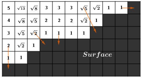
Given some mesh or a mesh-based scene, the difficult part is actually calculating the distance field. In the case of static scenes, this could be done in advance. In the example on the right you can see such a pre-calculated distance field of an object. It is a 3D field and the example shows it one slice at a time. The interior of the mesh is colored blue. You can try to guess how that object would look like in 3D. We will see it later on in an actual render.
There is not too much to say about distance fields by themselves in the context of fractals. We will be using distance fields, or more precisely, distance estimator functions in 3D fractal rendering with ray marching.
Links
- Distance Fields – Philip Rideout
Algorithms for generating distance fields. - mesh_to_sdf Python library
Useful to easily create an SDF for a given mesh.
Ray Marching
To render 3D escape time fractals we will use a rendering technique called ray marching. Note that we do not have a polygonal surface here, so the regular standard graphics pipeline rendering will not work. We also cannot do the regular ray tracing solution as our surfaces are complicated – they are not standard shapes like spheres and triangles that have known formulae for calculating intersection points with a ray. Instead, we have an arbitrary surface and a distance field that tells us the closest distance to it.
The ray marching technique does consist of shooting a ray into the scene, so the initial setup is the same as with ray tracing (we set up an origin and a direction for each camera ray). However, each ray then takes a number of steps while traversing the distance field. The size of the step will be the value read from the distance field. The ray marches along the field.
We will either march the ray some maximum number of times or until we reach the surface. Reaching the surface usually means the next step would be smaller than some specific length. In the picture above the space is divided into quite big voxels, so there will be some noticeable errors and we could check for exactly $0$. In usual cases, the smallest possible ray march distance could be a configurable small value. The bigger we make it, the more surface detail we will lose, but the faster the rendering.
When we hit a surface, we can color the pixel some single color. You can imagine that this will result in a pretty 2D-ish image. We will look at how to get a surface normal a bit later. One easy thing we can do to make the result look more 3D is to add ambient occlusion (AO). This is very easy to do with this rendering technique: We just add some black depending on how many steps the ray made. The more steps it makes, the more likely it entered some crevasse or hits the surface at a grazing angle. When we color such areas darker, we get a more 3D look.
We can ray march a pre-existing distance field, like the one from the Distance Field material before, or we might have a mathematical distance estimation (DE) function. One easy way to render a sphere would be to create a distance field $DE(p) = length(center - p) - radius$. The further along we are from the surface, the larger our values will be, the surface is defined at some distance $radius$ from the point $center$ and the function will be $0$ there. We could create many shapes in a similar fashion and combine them together with smooth operators as shown by Inigo Quilez.
In the example to the right, we have the distance field from the Distance Field material, which is now visualized via ray marching. It is a Doll! You can switch to the Balls demo to see the result of evaluating a mathematical distance estimation function during the march. You can turn the AO on and off. When you visualize the iteration count instead of rendering the shape, you can see that rays that barely pass the shape also have larger counts (the darker areas around the shapes).
Links
- Raymarching Distance Fields (2008) – Inigo Quilez
Great site of things related to the topic. There is also a site index with these and other topics. - Ray Marching – Michael Walczyk
Overview of ray marching with code examples, good illustrations, and surface normal estimation.
Box and Sphere Folding
Now that we can render arbitrary 3D objects as long we know a distance estimation function, we can start thinking about 3D fractals. There is a famous Mandelbrot analogue for 3D called the Mandelbulb. In this material, however, we will be creating a fractal called the Mandelbox. It will take a bit of doing to create the Mandelbox process function and then a distance estimation function. We will start with the pieces of the former – the box and sphere fold operations.
Box Folding
This operation starts kind of like folding a piece of paper into a box shape. We do not end at a 3D box shape but keep folding on until we get back to a 2D piece of paper. You can already imagine that this would be impossible in the real world. And we will be doing it in 3D!
We first define some folding distance $d$. Some points in the space will be less than $-d$ (blue), some will be greater than $+d$ (green), and some will be between $-d$ and $+d$ (red).
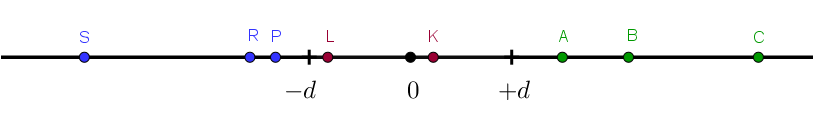
The points we have drawn here are just some reference points. It is the whole axis below $-d$ or above $+d$ that will fold.
Note that after this operation the area $[-d, d]$ will have more points mapped to it than before.
Mathematically you could also think of this as two conditional reflections. All the points less than $-d$ will reflect over $-d$ and all the points greater than $+d$ will reflect over $+d$.
This is also the idea behind how you would implement it.
void boxFold(inout vec3 z, float d) {
    z.x = abs(z.x) > d ? sign(z.x) * 2.0 -z.x : z.x;
    z.y = abs(z.y) > d ? sign(z.y) * 2.0 -z.y : z.y;
    z.z = abs(z.z) > d ? sign(z.z) * 2.0 -z.z : z.z;
}
Or you could write the if statements out:
void boxFold(inout vec3 z, float d) {
    if (abs(z.x) > d) { z.x = sign(z.x) * 2.0 - z.x; }
    if (abs(z.y) > d) { z.y = sign(z.y) * 2.0 - z.y; }
    if (abs(z.z) > d) { z.z = sign(z.z) * 2.0 - z.z; }
}
If you do not like conditions, then you could write the same thing very shortly as just:
void boxFold(inout vec3 z, float d) {
    z = clamp(z, -1.0, 1.0) * 2.0 - z;
}
Feel free to check that all these are mathematically equivalent and produce the correct result.
Sphere Folding
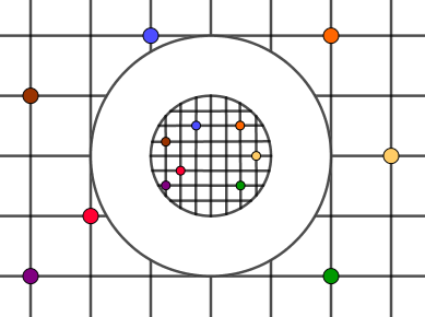
The next useful operation will be sphere folding. Assume we start with a grid with some points on it for reference. We use a grid to better see how the entire space transforms. For sphere folding, there are two circles centered at the origin: a smaller circle with radius $r$ and a larger circle with radius $R$. These radii will be parameters to the operation just like the folding distance was a parameter of the box folding.
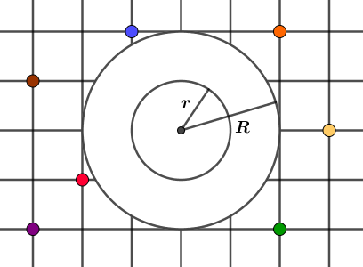
First, we are going to fill the smaller circle. We fill it with the downscaled version of our space. The scale factor will be $R^2 / r^2$. In our current example $R = 2$ and $r = 1$, so the inner circle will be filled with our space downscaled $2^2 / 1^2 = 4$ times. You can notice that our reference points also appear in the downscaled space. This is a very obvious source of a fractal-like structure – a larger and a smaller version of the same space occur simultaneously
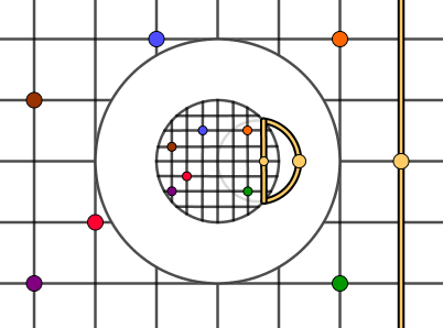
Second, we want to fill in the band between the smaller and larger circles. Mathematically what will happen there will be a circle inversion (in 3D sphere inversion) of the outer space against the larger circle. All the points will be reflected over the circle in a specific way. Because our point is in the origin, the condition will be $|p'| = r^2 / |p|$, where $p$ is our initial point and $p'$ is the point projected over the circle. If we want to operate with coordinates, then the formula to transform a point would be $p' = p * r^2 / (x^2 + y^2) = p * r^2 / p \cdot p $.
In the following picture, we have found an inversion for the yellow reference point and the vertical line that passes it. Note that all the other points on the yellow vertical line will be further away from the circle's border (if we move up or down on the line). Thus their inversions will also be further away. The result will be (a part of a) circle. One of the properties of circle inversion is that all lines become circles in the inversion.
Let us invert all the vertical lines.
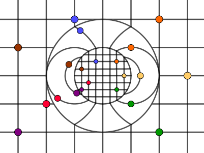
Because we previously chose the scale factor for space in the middle circle to be $R^2 / r^2$, then we get a pretty cool image, where the lines are connected with their counterparts in both circles. For example, take the line with the blue reference point on it. If you start from the top, you follow the vertical line to the blue dot in the outer space. Then the line goes to the circle inversion band where we meet our blue dot again. Following the line, we end up in the inner circle with the downscaled space. After meeting a third copy of the blue point. The line will then lead us out of the inner circle, through the circle inversion band, and then to the bottom of the picture.
For the complete picture, we also add the inversions of the horizontal lines.
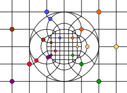
This is the complete sphere fold operation. It creates an interesting locally repeating (folded) effect. Note that the points further away actually will not be visible inside the circles. If a point is further than roughly the purple point is, it will be outside the small circle radius in the downscaled copy. In the circle inversion part, it would also go outside the band. If we would only have the circle inversion (and no small circle for the downscaled space), then all the outer space would be projected into the circle. But because it is a band, then all the space further away will be cut off in the inversion by the small circle.
On the right, there is an example, where you can play around with the radii. It might be useful to make it fullscreen so the (generated) grid pattern would not get too much Moire aliasing. The last slider can be used to quickly hide the sphere folding for seeing the underlying texture. Notice that already with this we can create some really cool fractal images. If you change $r$ to $0$ (and $R \neq 0$), then all of the infinite space will get packed into the only remaining circle.
Code-wise the implementation could be something like this:
void sphereFold(inout vec2 p, float r, float R) {
    float len2 = dot(p, p);
    float r2 = r * r;
    float R2 = R * R;

    if (len2 < r2) p *= R2 / r2;
    else if (len2 < R2) p *= R2 / len2;

    // You could also calculate the sphere-folded coordinates this way:
    //else if (len2 < R2) p = normalize(p) * R2 / length(p);
}
Of course, instead of the inout keyword, you could also just return the new coordinates here and in the box folding code before.
Later we will be using box folding and sphere folding in 3D for defining the Mandelbox fractal. Mathematically these operations are also called conditional scaling.
Automatic Differentiation
When we want to ray march a surface, we will need its distance estimation function. Remember from the Distance Fields chapter before that, at each location we need to know the distance to the nearest surface point of the shape we want to render. When we have functions $\mathbb{R}^3 \Rightarrow \mathbb{R}$, we can define a surface at $f(p) = 0$ for example. Such surfaces are called level surfaces (there is a surface when the value of a function is at some level, at level $0$ in our example). So, we need to find a distance between our current point $p$ and the closest point on the surface $p_c$.
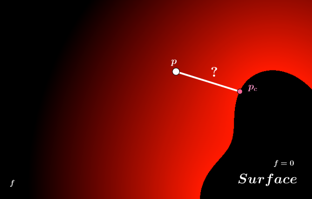
Note that we know $f$, it is the function whose values we use to define the level surface, but it is not the distance function. We do not know how the function $f$ behaves. But we can evaluate $f$ at $p$ or $p_c$ and get a number. What we are interested in is that is the shortest distance to the surface, ie, $|p_c - p|$, but we do not know where $p_c$ is. All we know about $p_c$ is that it is approximately the closest point to $p$, where $f(p_c) = 0$.
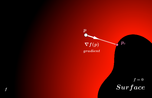
To get to $p_c$ we need to know how the function $f$ changes around $p$. Which way does the function get closer to the surface? Which way would we be moving away from the surface? More specifically we want to know, in what direction would we move fastest towards the surface and thus to $p_c$?
That will be the gradient of $f$ at $p$. Written out it is:
$\nabla f(p) = \begin{pmatrix} \nabla f(p)_x \\ \nabla f(p)_y \\ \nabla f(p)_z \end{pmatrix} = \begin{pmatrix} \delta f(p) / \delta x \\ \delta f(p) / \delta y \\ \delta f(p) / \delta z \end{pmatrix}$
All this taunting notation says is that it is a vector, where each coordinate shows how much the function changes when we change the corresponding ($x$, $y$, or $z$) coordinate of the input. We have found such gradients already during the Computer Graphics course in the Bump Mapping homework. There we used a finite difference method to find it, but here we will soon be using another approach to find it.
Assuming we have the gradient, we can approximate the closest distance to the surface by taking inspiration from a technique called the Newton's method. It is an iterative method that estimates the distance to the root of a function (where the value is $0$) via $f(p) / f'(p)$. One property of that technique is that closer we are to the actual root, the more accurate the estimation. So, it will be ok if we have a not-so-good estimation if our ray is still far away. We may make more steps, but when we are close to the surface, just one iteration of the Newton's method should be accurate enough. There is a small problem. The Newton's method is meant for $\mathbb{R} \Rightarrow \mathbb{R}$ functions. We have a $\mathbb{R}^3 \Rightarrow \mathbb{R}$ function. Thus, we need to use the Directional Newton's Method by Levin and Ben-Israel.
Intuitively the problem with an $\mathbb{R}^3 \Rightarrow \mathbb{R}$ function is that which way do we estimate the distance to $0$? We need to specify that we want the closest one, $f(p_c) = 0$, whose direction is given by the gradient. Generally, the formula for the distance estimation in direction $d$ with the Directional Newton's Method is:
$ \displaystyle{\frac{f(p)}{\nabla f(p) \cdot d} \cdot d} $
When we use the direction given by the gradient, we get:
$ \displaystyle{\frac{f(p)}{\nabla f(p) \cdot \nabla f(p)} \cdot \nabla f(p) = \frac{f(p)}{| \nabla f(p)| ^2} \cdot \nabla f(p)} $
Because we are only interested in the distance, ie, length of the approximation, we can do:
$ \displaystyle{\left | \frac{f(p)}{\nabla f(p) \cdot \nabla f(p)} \cdot \nabla f(p) \right | = \frac{|f(p)|}{| \nabla f(p)| ^2} \cdot |\nabla f(p)| = \frac{|f(p)|}{| \nabla f(p)| }} $
Note that $f(x)$ is a scalar here. The only vector (apart from $p$) is the gradient, which is why we could move the length calculation inside (bring the scalar out).
We need one more piece of the puzzle. Right now we only thought about the fact that our function outputs a single number in the end for a given 3D point. For escape-time fractals (like Julia and Mandelbrot, but also Mandelbox later on) our recursive process function is (most of the time) $\mathbb{R}^3 \Rightarrow \mathbb{R}^3$. This means that change in every one of the input coordinates could result in changes in any one of the output coordinates. We do not just have one number, but actually, three different numbers that change in the output. We will need a matrix to hold together the effects every input coordinate can have on every output coordinate (until we collapse them to a single scalar value). This is called the Jacobian matrix:
$J = \begin{pmatrix} \delta f_x(p) / \delta x && \delta f_x(p) / \delta y && \delta f_x(p) / \delta z \\ \delta f_y(p) / \delta x && \delta f_y(p) / \delta y &&\delta f_y(p) / \delta z \\ \delta f_z(p) / \delta x && \delta f_z(p) / \delta y && \delta f_z(p) / \delta z \end{pmatrix}$
It looks very scary, but you can just look at the different columns. The first column tells us what happens with our output point when $x$ of the input changes. The second column shows the output change when $y$ of the input changes. The last column does the same for input's $z$. You can also look at the rows. Each row shows the change of our function in only one coordinate. The rows are basically $\mathbb{R}^3 \Rightarrow \mathbb{R}$ gradients separately for output's $x$, $y$, and $z$ coordinates.
Fortunately, our escape-time fractals give out a length in the end. The length we use to determine if a point has escaped or not. So at one point, we will move back from $\mathbb{R}^3 \Rightarrow \mathbb{R}$. When we do that we will get again a gradient from our Jacobian. The way to transform the Jacobian back to a gradient, when the function takes the length of the point in the end, turns out to be:
$\nabla f(p) = \displaystyle{\frac{f(p) \cdot J}{|f(p)|}}$
If we now apply the Directional Newton's Method on the distance of the function, we get:
$ \displaystyle{\frac{|f(p)|}{|\nabla f(p)|}} = \displaystyle{\frac{|f(p)|}{ \displaystyle{\left | \frac{f(p) \cdot J}{|f(p)|}\right |} }} = \displaystyle{\frac{|f(p)|}{ \frac{1}{|f(p)|} \cdot |f(p) \cdot J|}} = \displaystyle{\frac{|f(p)| \cdot |f(p)|}{|f(p) \cdot J|}} = \displaystyle{\frac{|f(p)|^2}{|f(p) \cdot J|}}$
So, to find the distance to the nearest surface for ray marching a fractal, we will need to either find the Jacobian or at least account for the factors of the Jacobian that affect the output's length. In the next chapter, we will see how both of these solutions work with the Mandelbox. Before that, there is still one piece missing. We need a way to find the Jacobian (the three gradients).
Dual Numbers
The common ways to find a derivative (or the gradient, or the Jacobian – depends on the function we have) are:
- Analytical derivation. We work it out on paper. Very difficult.
- Finite Difference (FD) methods. The forward, backward, and central difference methods. We sample the neighborhood and find the differences in each direction. This is what we did in the Bump Mapping task. The issue is that we need to sample the function several times, resulting in the algorithm being run again as many times as we need to sample enough of the neighborhood (depends on the method used and dimensionality of the function). Also has an arbitrary step size, the choice of which could cause inaccurate results.
- Automatic Differentiation (AD). We will keep track of the running derivative and change it according to how the function changes. We can use dual numbers for this to make it quite simple to do.
Dual numbers are quite an easy concept by themselves. They are 2-dimensional numbers, like complex numbers, but instead of the imaginary unit $i$ they have an abstract unit $\epsilon$. The property of $\epsilon$ is that $\epsilon^2 = 0$. Of course $\epsilon \neq 0$. This makes $\epsilon$ a nilpotent. Here are a few examples of some dual numbers:
$(a + b\epsilon) ~~~~ a, b \in \mathbb{R}$
$(1 + 2\epsilon) + (5 + 2 \epsilon) = (6 + 4 \epsilon)$
$(1 + 2\epsilon) \cdot (5 + 2 \epsilon) = 5 + 2 \epsilon + 2 \epsilon \cdot 5 + 2 \epsilon \cdot 2 \epsilon = (5 + 12 \epsilon)$
Notice that with the last multiplication the $2\epsilon \cdot 2\epsilon$ term disappears because $\epsilon^2 = 0$. You can see that the real component has an effect on the abstract component, but the opposite is not true. The abstract component does not have an effect on the real component. This is different from complex numbers. There are calculation rules for doing AD with dual numbers.
It turns out to be quite easy to now use dual numbers to calculate the running first derivative. If we have a function we want to find the derivative for at certain values, we can just replace all our inputs and constants with dual numbers and the abstract part will store the first derivative. For example, if we have a simple function $f(x) = 3x^2$ we can get the value of the function and its first derivative at $4$ by using $(4 + 1 \cdot \epsilon)$ instead of $4$. It would follow:
$f(4 + \epsilon) = 3 \cdot (4 + \epsilon)^2 = 3 \cdot (16 + 2 \cdot 4 \epsilon) = (48 + 24 \epsilon)$
So $f(4) = 48$ and $f'(4) = 24$. No sweat. Note that the abstract part of the input should be $1$ if it is the input whose effect on the function's change (derivative with respect to it) we want to calculate. In the case of constants, the abstract part should be zero.
In the case of multivariate functions (functions with multiple inputs) $\mathbb{R}^n \Rightarrow \mathbb{R}$ we can find the gradient. For that, we use vectors in the abstract part that have $1$ in the place where we want to store the partial derivative of a specific variable for and $0$ elsewhere. For example, take a function $f(x, y) = 2 x + xy$. If we want to evaluate it and its gradient at $(5, 2)$, then we use $(5 + [1, 0]\epsilon, 2 + [0, 1]\epsilon)$. It follows that:
$f(5 + [1, 0]\epsilon, 2 + [0, 1]\epsilon) = 2 \cdot (5 + [1, 0]\epsilon) + (5 + [1, 0]\epsilon) \cdot (2 + [0, 1]\epsilon) = (10 + [2, 0]\epsilon) + (10 + [0, 5]\epsilon + [2, 0]\epsilon + 0) = (20 + [4, 5]\epsilon)$
So, the values are $f(5, 2) = 20$ and $\nabla f(5, 2) = [4, 5]$. Because this is a linear function, we can tell that if we are at $(5, 2)$ and we increase $x$ by $1$, then we increase the function's value by $4$, if we increase $y$ by $1$, we increase the function's value by $5$.
For completeness, we can now try the Directional Newton's method we described before. According to that, approximated vector to the closest point on the $0$-level surface would be $|f(5, 2)| / |\nabla f(5, 2)| = 20 / \sqrt{4^2 + 5^2} \approx 6.4$ units away. We can use WolframAlpha to find the actual root, which turns out to be $[0, -2]$, which is $\sqrt{(5-0)^2 + (2+2)^2} \approx 6.4$ units away like we estimated.
It will not always give the correct answer in the first iteration like that. Here are two other functions and results from several iteration steps:
| $x + y^2$ | $2x + xy$ | |||
| 1 | $(3, 4)$ | $19+ [1, 8]\epsilon$ | $(5, 2)$ | $20 + [4, 5]\epsilon$ |
| 2 | $(2.71, 1.66)$ | $5.47 + [1, 3.32]\epsilon$ | $(3.05, -0.44)$ | $4.76 + [1.56, 3.05]\epsilon$ |
| 3 | $(2.25, 0.15)$ | $2.28 + [1, 0.31]\epsilon$ | $(2.42, -1.68)$ | $0.78 + [0.32, 2.42]\epsilon$ |
| 4 | $(0.17, -0.48)$ | $0.40 + [1, -0.97]\epsilon$ | $(2.37, -1.99)$ | $0.01 + [~0, 2.37]\epsilon$ |
| 5 | $(-0.04, -0.28)$ | $0.04 + [1, -0.56]\epsilon$ | $(2.37, -2)$ | $~0 + [~0, 2.37]\epsilon$ |
| 6 | $(-0.07, -0.26)$ | $ ~0 + [1, -0.57]\epsilon$ | ||
We can see that it takes several steps from these chosen starting points to reach $0$. However, as we get closer, we get better steps. For example with $2x + xy$ from iteration 1 to 2 we have a decrease in the value by about 75%. But from iteration 3 to 4 it is about 99%. With ray marching it is not a big problem, we will just make a few more steps.
Finally, we can see what happens in the $\mathbb{R}^3 \Rightarrow \mathbb{R}^3$ case. We start similarly in that we use vectors for the abstract part of our inputs: $f(x' + [1, 0, 0]\epsilon, y' + [0, 1, 0]\epsilon, z' + [0, 0, 1]\epsilon)$. After calculating the function, we get out a 3D point that also has some abstract parts $f(p) = (x' + [a, b, c]\epsilon, y' + [d, e, f]\epsilon, z' + [g, h, i]\epsilon)$. The numbers, and thus the abstract parts, do not become one as they did before. Instead we have three gradients here. The gradient $[a, b, c]$ shows how the input $x$, $y$, and $z$ affect the output's $x$ coordinate. The other gradients are similar but with respect to $y$ and $z$ coordinates. You can probably already tell that these form the Jacobian:
$J = \begin{pmatrix} a && b && c \\ d && e && f \\ g && h && i \end{pmatrix} = \begin{pmatrix} \delta f_x(p) / \delta x && \delta f_x(p) / \delta y && \delta f_x(p) / \delta z \\ \delta f_y(p) / \delta x && \delta f_y(p) / \delta y &&\delta f_y(p) / \delta z \\ \delta f_z(p) / \delta x && \delta f_z(p) / \delta y && \delta f_z(p) / \delta z \end{pmatrix}$
Great, so all we have to do is calculate every part of our algorithm with dual numbers and we get out a Jacobian. From the Jacobian, we can get the gradient. Then we use that gradient in the Directional Newton's Method to estimate the distance to the nearest surface (in the direction of the gradient).
Implementation-wise we can pass along a vec3 for the real part and a mat3 for the Jacobian in the abstract part.
function fractal(vec3 p) {
    vec3 dp = mat3(1.0);

    for (int i = 0; i < maxI; i++) {

        doStuff(p, dp);

    }

    return dot(p, p) / length(p * dp); // The distance estimation via Directional Newton's Method. This is what we found just before starting the Dual Numbers subchapter.
}
Links
- Automatic Differentiation with Dual Numbers (2019) – Alejandro Morales
Easy to read introduction into AD and dual numbers. - Automatic Differentiation using Dual Numbers (2020) – Erik Engheim
Implementation example of AD with dual numbers. - How to Differentiate with a Computer (2017) – David Austin
Good explanation on how to use dual numbers for AD with the Newton Method. - A Hitchhiker’s Guide to Automatic Differentiation (2016) – Philipp H. W. Hoffmann
Comprehensive and scientific. - Directional Newton Methods in n Variables (2001) – Yuri Levin, Adi Ben-Israel
To estimate the distance to the surface in a given direction. - Math for Game Programmers: Dual Numbers (2013) – Gino van den Bergen
Interesting GDC talk about dual numbers and other stuff.
The Mandelbox
Now we are ready to construct the Mandelbox. It is an escape-time fractal, just like Julia and Mandelbrot were, but in 3D and with a different formula:
$z_{n+1} = sphereFold(boxFold(z_n)) \cdot scale + z_0 \cdot offset$
To render it, we need to estimate its distance function. Using dual numbers for this, we already know how to add and multiply different dual numbers. However, the box folding and sphere folding are worth looking into.
For the box folding, we reflect an axis over a constant when the absolute value of the coordinate is larger than some constant $d$. We can use conditionals with dual numbers. Thus, if we have a $p$, where we need to flip, we just multiply the whole dual number with $-1$. If gradients are in the rows of the Jacobian, then the code would be:
void boxFold(inout vec3 p, inout mat3 dp) {

    if (abs(p.x) > d) {
        p.x *= -1.0;
        dz[0].x *= -1.0; dz[1].x *= -1.0; dz[2].x *= -1.0;
    }
    if (abs(p.y) > d) {
        p.y *= -1.0;
        dz[0].y *= -1.0; dz[1].y *= -1.0; dz[2].y *= -1.0;
    }
    if (abs(p.z) > d) {
        p.z *= -1.0;
        dz[0].z *= -1.0; dz[1].z *= -1.0; dz[2].z *= -1.0;
    }

}
Parts of this could be optimized, written in vector form, etc, but mathematically we need to do for each axis $a \in [x, y, z]$:
$-1 \cdot (p_a + \nabla f(p)_a \cdot \epsilon)$, if $|p_a| > d$.
Or when write the gradient out:
$-1 \cdot (p_a + \left [\frac{\delta f_a(p)}{\delta x}, \frac{\delta f_a(p)}{\delta y}, \frac{\delta f_a(p)}{\delta z} \right]\epsilon)$, if $|p_a| > d$.
This makes sense as we change the direction of one axis, we change the direction of the output's corresponding coordinate.
With sphere folding it is more complicated. There are two branches, in the first we just multiply by a constant $R^2 / r^2$. That goes like regular scalar constant multiplication. However, in the other branch, we divide with $R^2 / |p|^2$. The proposed operation to perform on the all the columns of the Jacobian $J = |c_{fx}, c_{fy}, c_{fz}|$ in that branch is:
$\displaystyle{\frac{R^4}{|p|^4} \cdot \left ( c_i - p \cdot \frac{2 (p \cdot c_i)}{|p|^2} \right )}$.
The $p \cdot c_i$ is the dot product. The real number part we multiply with just $R^2 / |p|^2$.
Honestly, I have no idea where this comes from. It makes some sense as at sphere folding all the output coordinates depend on all the input coordinates. So it is logical to change all the elements of the Jacobian and account for the interplay. When using that code it seemed to give a better result by just multiplying the matrix with $R^2 / |p|^2$ instead of $R^4 / |p|^4$.
Code-wise sphere folding (with my replacement) would be:
void sphereFold(inout vec3 p, inout mat3 dp) {

    float len2 = dot(z, z);

    if (len2 < r2) {

        float s = R2 / r2;
        multiplyScalar(p, dp, s);

    } else if (len2 < R2) {
        float s = R2 / len2;

        dp[0] = dp[0] - p * 2.0 * dot(p, dp[0]) / len2;
        dp[1] = dp[1] - p * 2.0 * dot(p, dp[1]) / len2;
        dp[2] = dp[2] - p * 2.0 * dot(p, dp[2]) / len2;

        multiplyScalar(p, dp, s);
    }
}
When these functions are good, then all that is left is the main iteration:
function mandelbox(vec3 p) {
    vec3 dp = mat3(1.0);
    mat3 dc = dz;
    vec3 c = z;

    for (int i = 0; i < maxI; i++) {

        boxFold(p, dp);
        sphereFold(p, dp);
        multiplyScalar(p, dp, scale);
        add(p, dp, c * offset, mat3(0.0)); // Instead of mat3(0.0) there should be "dc" here, but that caused a lot of aliasing and a lumpy fractal

    }

    return dot(p, p) / length(p * dp); // The distance estimation via Directional Newton's Method. This is what we found just before starting the Dual Numbers subchapter.
}
This will render you a Mandelbox, but it will be quite flat-looking. You could add ambient occlusion, but what we really want here are the surface normals.
We could get the surface normals with a finite difference method, which would need us to sample the mandelbox function more times. However, we can observe that when we hit the surface of a fractal, we always do it in the same direction as the gradient. So we could just take the gradient to be our surface normal. In principle, this should be the negated gradient, but for some reason, it is the positive gradient that works for me.
$\displaystyle{normal = \frac{f(p) \cdot J}{|f(p) \cdot J|}}$
In code we would thus have:
function mandelbox(vec3 p) {
    vec3 dp = mat3(1.0);
    mat3 dc = dz;
    vec3 c = z;

    for (int i = 0; i < maxI; i++) {

        boxFold(p, dp);
        sphereFold(p, dp);
        multiplyScalar(p, dp, scale);
        add(p, dp, c * offset, mat3(0.0));

    }

    return deResult( // This could be a struct
        dot(p, p) / length(p * dp),
        normalize(p * dp)
    )
}
There is an alternative solution, which would just keep track of the Jacobian changes the magnitude of the distance to the closest surface. For that, we will first analyze the final distance calculation from the previous approach:
$\displaystyle{\frac{|f(p)|^2}{|f(p) \cdot J|}}$
Keep in mind that we are only interested in the distance and assume that the Jacobian changes the distance of a vector by some specific value $a$ when multiplied from the left. Then we would have:
$\displaystyle{\frac{|f(p)|^2}{|f(p) \cdot a|} = \frac{|f(p)|^2}{|f(p)| \cdot |a|} = \frac{|f(p)|}{|a|}}$
Now, all we need is to check if our assumption is correct and then know the value of $a$. Our Mandelbox process starts with a unit Jacobian. You can think of it as a scale matrix with the scale factors being all $1$. Then we are doing box folding. That operation only changes the sign of one row, so does not make the Jacobian scale anything bigger or smaller. Next, we have sphere folding. For that we need to analyze what is happening when we do:
$\displaystyle{\frac{R^2}{|p|^2} \cdot \left ( c_i - p \cdot \frac{2 (p \cdot c_i)}{|p|^2} \right )}$.
Note that here we use $R^2 / |p|^2$ as this is also what I use in the code.
$\displaystyle{\frac{R^2}{|p|^2} \cdot \left ( c_i - p \cdot \frac{2 \cdot |p| \cdot |c_i| \cdot \cos(\angle{p, c_i})}{|p|^2} \right ) = \frac{R^2}{|p|^2} \cdot \left ( c_i - \frac{p}{|p|} \cdot 2 \cdot |c_i| \cdot \cos(\angle{p, c_i}) \right ) = \frac{R^2}{|p|^2} \cdot \left ( c_i - 2 \cdot \hat{p} \cdot (\hat{p} \cdot c_i) \right ) }$.
Here $\hat{p}$ is normalized $p$ and $\hat{p} \cdot c_i$ is the dot product. What we find is that this is reflecting the column of the Jacobian over our vector $p$. As it is a reflection, it does not change the length of $c_i$. Meaning that the Jacobian here will become a rotation matrix, but all the axes still have the scalar factor just $R^2 / |p|^2$.
In the other sphere folding branch, there is only scaling with the scalar factor $R^2 / r^2$.
We then multiply with $scale$, which also would multiply the Jacobian. Lastly, we add the $offset$, which with our mat(0.0) does not add anything to the Jacobian.
Thus, if we are only interested in the closest distance, then we could substitute the Jacobian matrix with just a running scalar value $a$:
void add(vec3 p, float a, vec3 q, float dq) {
    // Add dq to a
    // (in our case dq is 0, so we do nothing)
}

void multiplyScalar(vec3 p, float a, float s) {
    // Multiply a with s
}

void sphereFold(vec3 p, float a) {
    // Multiply a with either
    // R^2 / r^2
    // or
    // R^2 / |p|^2
}

void boxFold(vec3 p, float a) {
    // do nothing with a
}

function mandelbox(vec3 p) {

    vec3 c = z;
    vec3 dp = mat3(1.0);
    mat3 dc = dz;
    float a = 1.0;


    for (int i = 0; i < maxI; i++) {

        boxFold(p, dp a);
        sphereFold(p, dp a);
        multiplyScalar(p, dp a, scale);
        add(p, dp a, c * offset, 0.0);

    }

    return deResult(
        dot(p, p) / length(p * dp),
        normalize(p * dp)
        length(p) / abs(a),
        normal
    )
}
This is how the code from many Mandelbox implementations like the one in this Shadertoy comes from.
The only issue here is that we do not have the information to assess the normal anymore. Thus solutions like that usually use a finite difference method to assess the normal, resampling the distance estimation function several times at nearby coordinates.
On the right, there is an example with the Mandelbox. The example is split into two. The left part of the screen shows the simplified version, where normals are estimated by a finite-difference (FD) method. The right part is the implementation with the Jacobian matrix, where the normal is calculated from the gradient vector directly. The first slider (FD/AD cutoff) controls the split. The second slider (Cam Z) controls. The next two sliders (Hit Min/Max Dist.) control the distance from where a ray is considered to be on the surface. Then come the sphere fold sliders (Min/Max Radius), the scale parameter (MB Scale), and the box fold parameter (Box Fold Dist.).
Notice that the FD and AD solutions do not produce completely identical pictures. There are weird circular artefacts in the AD solution, which are especially obvious if you increase the Hit Min Dist. to around 0.29 and zoom out.
At the bottom of the example, there are a few saved scenes (parameter configurations) to check out.
If you want to explore the Mandelbox further, then both the AD and FD versions are available in Fragmentarium and this site has Mandelbox parameters for Mandelbulber 2.
Links
- Distance Estimated 3D Fractals (VI): The Mandelbox (2011) – Mikael Hvidtfeldt Christensen
Good overview of what the Mandelbox is and also derives the running scalar factor solution. - Distance Estimated 3D Fractals (VII): Dual Numbers (2011) – Mikael Hvidtfeldt Christensen
The main article used in the Mandelbox chapter here. - The Mandelbox, an Artistic and Geometric Journey – Torsten Stier
Several cool places inside the Mandelbox. - Mandelbox – Tom Lowe
A website dedicated to the Mandelbox (use the menu on the top-left) - The Mandelbox Set (2014) – Rudi Chen
Mathematical dive into the Mandelbox. - A Mandelbox Distance Estimate Formula (ca 2010)
The FractalForums thread of when people were discovering the Mandelbox. - Mandelbox Fractals and Flights (2015) – Mark Craig
Explanation and flythrough videos of the Mandelbox. - Extending Mandelbox Fractals with Shape Inversions (2018) – Gregg Helt
What happens if you extend the sphere fold into shape inversion and use some other shapes.