Post-Processing Effects
Many visual effects can be done on the frame after it has been rendered. Due to that, they are called post-processing effects. You could even think about these in terms of photography. In professional photography, the picture you take with the camera is just the base. That picture is then modified in Adobe Photoshop, Affinity Photo, Corel PaintshopPro, or other photo editing software. Some of the things you might do would be to increase the contrast, perhaps use the Levels or Curves tools for fine contrast and brightness control. Perhaps you make it sharper using the Sharpen or Unsharp Mask tools. In computer graphics, post-processing effects have a similar goal. We have our base render, and we want to make it somehow better.
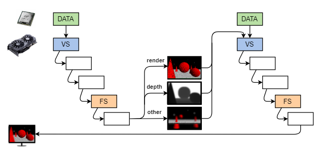
From the standard graphics pipeline, we not only get the rendered frame, but we could have many other inputs to a particular post-processing effect. Of course, scene depth could be one of them. But we could also have certain objects or layers in the scene rendered separately. Not only that, but the entire post effect could also take several passes to complete. This is similar to what we also saw in the Deferred Rendering topic before.
In this topic, we look at some specific effects and tools that are used to make them. Of course, there exist many effects and many approaches to achieve a particular effect.
Definitions:
- Post-processing effect – An effect that is applied to a frame once the scene (or part of it) has been rendered to it.
- Convolution – Technique that combines two signals (images). Used in several image filters.
- Kernel – Matrix that is used as the second argument in convolution filters.
- Separable kernel – Kernel that can be represented as a multiplication of a row and a column matrix.
- Symmetric kernel – Kernel that exhibits some symmetry (eg, vertical, horizontal, circular).
- Singular Value Decomposition – Technique that decomposes one matrix into three specific matrices.
Convolution
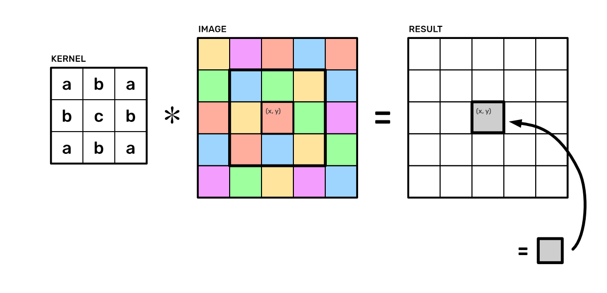
Image processing techniques like sharpen and blur are based on a signal processing technique called convolution. Generally, convolution is an operation between two signals, combining them into one. In image processing, our signals are images, which are matrices of numbers. Thus we have 2D discrete convolution. The convolution operation has a symbol $∗$. We use it to combine together our image $\text{P}$ and a smaller image $K$ called a kernel or filter. The kernel is usually a square with an odd width and height. We could define a radius $r$ for it such that $width = 2r+2$. In such case, the result of the convolution for a specific texel of the image $\text{P}$ at $(x, y)$ would be:
$$\Large \text{K}∗\text{P}(x, y) = \sum_{\Delta x=-r}^{\Delta x=r} \sum_{\Delta y=-r}^{\Delta y=r} \text{K}(-\Delta x, -\Delta y) \cdot \text{P}(x + \Delta x, y + \Delta y)$$.
Intuitively what is happening is that for one pixel, we lay the kernel on top of it (thus the odd size of the kernel). Then we mirror the kernel in width and height, sample the image from underneath all the kernel's elements, multiply those samples with the kernel values, and finally sum all of that together for the pixel's new value. The confusing part here is the mirroring of the kernel, which has its origins in signal processing. There is another operation called correlation, which does not mirror the kernel. Also, if our kernel is circularly symmetric, then $\text{K}(-\Delta x, -\Delta y) = \text{K}(\Delta x, \Delta y)$ and we can omit the mirroring. In such cases, we can visualize the convolution like this:
One of the simplest forms of blur could be done via convolution by just having $1/9$ in each of the elements of a $3×3$ kernel. That is called box-blur, as it leaves a box-shaped aliasing in the blur because of the shape of the kernel. You could also call it the mean filter, as it takes the mean of the neighboring pixels.
The Laplacian Kernel
Another thing we could try to do is sharpen the image. The tool Unsharp Mask gets its name from its original conception of adding to the image a difference between a blurred (unsharp) and an original version of the image. The idea is that we will be looking for the second derivative of the image and adding it. Several different filters try to approximate the second derivative and sharpen the image. Here we are going to look at the standard Laplacian filter.
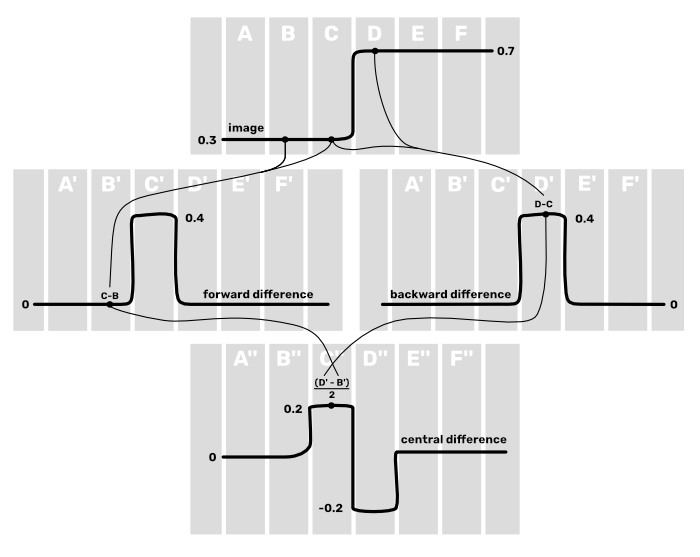
To derive it, we can first think about using the central difference method for approximating a derivative. Assume we have a 1D case with pixel values $\text{A}$, $\text{B}$, $\text{C}$, $\text{D}$, $\text{E}$, and $\text{F}$. If we would want to know the second derivative $\text{C}^{\prime\prime}$, it would be $\text{C}^{\prime\prime} = (\text{D}^{\prime} - \text{B}^{\prime}) / 2$. Okay, so we need to know $\text{D}^{\prime}$ and $\text{B}^{\prime}$. However, if were to use the central difference method again for those, we would also need to sample $\text{A}$ and $\text{F}$. So, we can do a small trick and just use the forward difference for $\text{B}^{\prime}$ and the backward difference for $\text{D}^{\prime}$. In that case $\text{B}^{\prime} = \text{C} - \text{B}$ and $\text{D}^{\prime} = \text{D} - \text{C}$. With this approach, all the samples need to use for approximating the second derivative $\text{C}^{\prime\prime}$ are just $\text{B}$, $\text{C}$, and $\text{D}$.
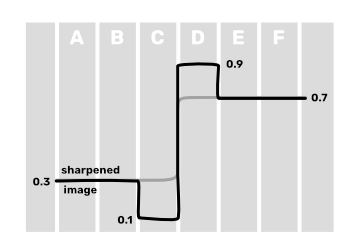
When this is done, then we can enhance the original image by subtracting the second derivative from it. What that would do is at the areas where there is an edge, change the lower side of the edge to be a bit lower and the higher side of the edge to be a bit higher. Thus it will create more contrast near that edge, making the image look sharper.
If we now write out how to combine $\text{B}$, $\text{C}$, and $\text{D}$, we would get that $\text{C}^{\prime\prime} = (\text{B} - 2 \text{C} + \text{D}) / 2$. We could regard the division by $2$ as a scalar factor, affecting how much we sharpen the image. Thus without it, our coefficients would be $1 \text{B}$, $-2 \text{C}$, and $1 \text{D}$. Because we want to subtract, we can negate these coefficients. We also are in 2D, meaning the same process would need to apply horizontally and vertically. Finally, because we want to combine the second derivative approximation with the original image, we can add one to the coefficient of $\text{C}$ (our current pixel). This is how the Laplacian filter below comes to be:
| Box Blur | Laplacian | ||||||||||||||||||
|
|
In the example to the right, we have a sphere with some procedural detail on it. The Noop (no-operation) filter does nothing. The Box filter applies the naive blur, where every pixel becomes an average of itself and its neighborhood. The Laplacian filter sharpens the image. It currently has no scale coefficient. You can think about how you would create a parameter that would change the effect intensity for each of these filters. Such that the blur and sharpening would have a smaller or a larger effect. Would it be possible in all cases, or what would you need to make it?
Links
- Digital Image Processing, 4th Editon (2017) – Rafael Gonzalez and Richard Woods.
The main textbook when it comes to all things related to image processing.
Blur
The box blur we saw before has a couple of issues. First, it has an unnatural box shape. We would rather want some circular shape such that the blur would be uniform in all directions. Perhaps having a larger kernel that takes the mean value of a disc, then? That would work, but this leads us to our second problem. Increasing the effect size for filters like blur increases the number of samples with square complexity. Even with the regular box blur, if we want to increase the size of the blur, the next kernel would be $5×5$ and would require $25$ samples. After that, we would have $7×7$ with $49$ samples and $9×9$ with $81$ samples. This is way too many samples in one frame for a simple post-processing effect.
Separable Kernels
Luckily there is a way to optimize this in some cases. You might remember from your algebra class that multiplying together two vectors can result in a matrix:
|
$\cdot$ |
|
$=$ |
|
Note that all the rows and columns are linearly dependent. The rank of such a matrix is 1. If we were to span a vector space (use these columns as the basis vectors), it would result in a 1D space. You can replace all the letters with some small numbers to see better that every row and column is a multiple of every other row or column. So, the set of such matrices that can be represented as a multiplication of two vectors is limited. However, there might still be some kernels that could be factored this way. If we look at our box blur filter, that is certainly a rank 1 matrix. The Laplacian, however, is not.
Let us also look at what happens if we perform the convolution between the same two vectors. To convolve those vectors, we need to set the values outside of the range to $0$. This is a common assumption when sampling outside a range. Secondly, we have to remember that convolution matches together the elements symmetrically around the center of the kernel. Meaning that in the calculation below, the top-left element would be calculated as $\text{a} \cdot \text{d} + \text{b} \cdot 0 + \text{c} \cdot 0$.
|
$∗$ |
|
$=$ |
|
Turns out that convolution between those two vectors gives the same result as multiplication. So, if our kernel could be separated into two vector factors, we have:
$\text{K}∗\text{P} = (\text{v}_0 \cdot \text{v}_1) ∗ \text{P} = (\text{v}_0 ∗ \text{v}_1) ∗ \text{P}$
One property of convolution is that it is associative. So, instead of doing convolution with the entire $n×n$ kernel, we can do two convolutions with 1D kernels of length $n$. This results in linear complexity instead of the original quadratic complexity:
$\text{K}∗\text{P} = \text{v}_0 ∗ (\text{v}_1 ∗ \text{P})$
Such kernels, which can be factored into two vectors, are called separable kernels. And now we could do quite large box blurs by first doing a horizontal blur, followed by a vertical blur.
The example on the left allows you to do box blur with kernels $63$ elements in length. Doing $2 \cdot 64 = 128$ samples per frame is still doable, while $64^2 = 4096$ would be extremely costly. The value in the vector kernels is just the square roots of the number of filled elements. You can think about what vectors would multiply together for the expected square kernel.
However, you can see that when the blur kernel becomes bigger, the box shape of the filter becomes quite apparent. Of course, this could be visually interesting, depending on the desired visual style. Still, most of the time, we would expect a more circular and uniform blur.
Gaussian Blur
If you think about circular shapes, you find out that a kernel with a filled disc calculating the mean (like our box kernel, but disc-shaped) would not be separable. The rows and columns would not be multiples of each other. In fact, there are almost no circularly symmetric separable real-valued kernels except one. The one that works is called a Gaussian kernel, and, just like the name says, it holds the 2D Gaussian function:
$\text{G}(x, y, \sigma) = \dfrac{1}{2\pi\sigma^2} \cdot \exp{\left(-\dfrac{x^2 + y^2}{2\sigma^2}\right)}$
Here $\sigma$ is the standard deviation, which we can change to change the width of the kernel, thus the size of the blur effect. Below are some kernels, which are normalized for displaying here such that their peak value would equal one. Note that while the kernels look small here, there are very small values in the visibly black areas too.
For use in the Gaussian blur, you would normalize the elements such that their sum equals one.
Now, to separate the kernel, you could pick any (for the model row) and then divide all the rows with that row, getting the coefficients for the other factor. However, here we show another, perhaps a bit overkill, trick. There is an operation called singular value decomposition (SVD), which decomposes a matrix into three specific matrices $\text{U}$, $\Sigma$, and $\text{V}^\text{T}$. These three matrices multiplied together give back our original matrix.
$\text{K} = \text{U} \Sigma \text{V}^\text{T}$
We are interested in the matrix $\Sigma$, which is a diagonal matrix that holds singular values. The number of non-zero singular values equals the rank of the matrix. Thus, if we have a separable kernel, SVD gives us only one singular value.
| K = |
$\text{U}$
|
$\cdot$ |
singular values $\Sigma$
|
$\cdot$ |
$\text{V}^\text{T}$
|
Note that because there is only one singular value in $\Sigma$, multiplying $\text{U}\Sigma$ or $\Sigma\text{V}^\text{T}$ would respectively give us a column and a row vector. If we now factor the singular value $\text{s}$ into two, then we have the kernel separations. Of course, we could just take the factors $\text{s}$ and $1$, which would give us the kernel separations as $\text{su}$ and $\text{v}$. However, it turns out that if the kernel can be separated into two identical factors, which is only when $\text{K}=\text{K}^\text{T}$, then the first column of $\text{U}$ and the first row of $\text{V}^\text{T}$ are also identical ($\text{u}_{i,0} = \text{v}_{0,i}$). So, in our case, the separations would be $\sqrt{\text{u}\text{s}} = \sqrt{\text{s}}\text{v}^\text{T}$:
| K = |
|
|
$\cdot$ |
|
|
So now, we can use the following rows shown in the picture below as the separated Gaussian kernels. Just like with box blur before, we would do convolution with a horizontal kernel separation, followed by the vertical one.

This is done in the Gaussian blur example to the right. You can see that this looks like a bit more natural blur than what we had before. We are not getting the box-shaped aliasing anymore, but the blur is applied in all directions equally.
As a side note, we mentioned that there are no other real-valued circularly symmetric separable kernels. However, if we extend our number space to complex numbers, we could create a separable kernel that approximates a solid disc. This would give us an even better blur, which would resemble more how camera lenses work. That approach has been implemented in several high-fidelity games like the Madden and Fifa series.
Links
- The Singular Value Decomposition (2011) – Allan Jepson, Fernando Flores-Mangas
Course material explaining the uniqueness of SVD results on page 4. - Proof of Associativity of Convolution (2017) – epi163sqrt
Stackexchange post proving the associativity of convolution. - Circular Separable Convolution Depth of Field (2017) – Kleber Garcia
The paper describing how separable disc-shaped blur was used in Madden games. - Video Game & Complex Bokeh Blurs (2019) – Computerphile
Video explaining the separable disc-shaped blur technique.
Depth of Field
Many visual effects in computer graphics are inspired by the visual effects people are accustomed to seeing in movies and photography or even how the human visual system works. One such effect is the Depth of Field (DoF). To understand it, we can look at how our eyes and cameras capture light. Both of them are based on the idea that we use a lens to capture light from an area and focus it down on a sensor. This means that to see one surface point $\text{P}$ we not only collect the light that directly travels from it via one light ray, but rather we collect many light rays that are slightly spread out.
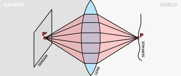
This allows us to capture more light and see the world better. Of course, increasing the size of the lens also helps. Nocturnal animals often have bigger eyes that can see more in the dark. To capture light from distant astral bodies, we build huge telescopes. Another option would be to increase the sensitivity of the sensor, but this can lead to a more noisy image. You have probably seen this when you have increased the sensor sensitivity (ISO) of digital photo cameras.
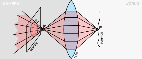
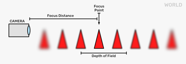
Unfortunately, this lens-based visual system has a problem. Namely, only a small area can be in focus at a single time. If we move our surface point $\text{P}$ closer to the lens, we can see that the projection $\text{P}^{\prime}$ is now no longer on the sensor. In fact, the focus point is in front of the sensor. The captured light rays from $\text{P}$ converge and then spread out again. On the sensor, we will see a blurry image of the point $\text{P}$. That blurred circular area is also called the Circle of Confusion (CoC).
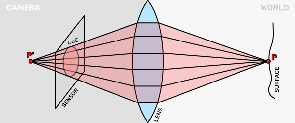
A similar thing happens when our surface is too far away from the camera. In that case the focus point $\text{P}^{\prime}$ would be behind the sensor. The sensor captures the rays before they can converge, thus we get a similar blurry image again.
Here we looked at how a single point got spread out on the sensor. There are many points in the scene, scattering light rays, and contributing to the image the sensor ultimately captures.
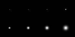
In photography, the term Depth of Field signifies the range in which objects are considered to be in focus (sharp). Different lenses and zoom levels produce different depths of field. This effect has become so familiar to us that we even intuitively recognize photographs or movie stills to be of small objects when they have a large depth of field. Or, if we have a photograph of something far away and there is something blurry in the foreground, we feel it being very close to the camera.
In our standard rendering pipeline, however, our approach to rendering is quite different. Our virtual camera does not have a lens that would capture the scattered light from an area. Rather, we just have a single point to which we project all our scene objects. It is effectively just capturing and rendering the straight light rays from every scene point. So, we use post-processing to add that effect to our scene.
The first thing to notice is that we have a varying level of blur depending on the distance from the focus point. Seeing as before we also had different kernels for blur, we can just make the choice of the kernel to be dependent on the scene depth. If the scene depth becomes less than some threshold, we start blurring the pixels and increasing the blur the smaller it gets. That would be the foreground. If the scene depth becomes larger than some other threshold, we again start blurring and increase it the larger it gets.
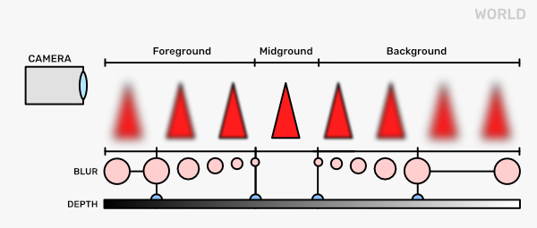
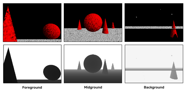
This is fine until we have just one object in our scene. As soon as we have several objects at different depths that cover each other, we start noticing issues. For example, when we are blurring a foreground object pixel, the blur kernel could also sample from the mid- or background objects. This would be wrong as these pixels are not at a similar depth. Or, when we blur the foreground object, its silhouette becomes transparent. This means that some of the previously solid pixels become transparent. Thus, we need to know what is behind them. If we just render our scene in one go, this information would be lost. Thus, the solution is to render the scene in layers. We separate out the foreground, midground, and background, then render and blur them all separately. When doing that, we need to make sure that we are not overwriting the pixel values with the ones outside of the current layer. For example, in the image below, you can see that while there is a big red cone on the left side of the foreground, the midground and background framebuffers hold the pixel values behind that cone.
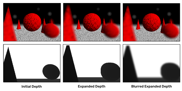
When blurring the layers, we can notice another issue. If we decide the blur size based on the depth of the current pixel, we can only blur inside the shapes. Think about the red foreground cone again. We want its silhouette to blur and spread out from its original position. However, the pixels just outside its original shape have either infinite depth or some other larger value than on the cone itself. Thus, the pixels just outside it get blurred very little if at all. One way to try to alleviate this is to expand the depth of the foreground objects. We could do this via a few iterations of the jump flood algorithm described in the NPR topic. Because this will still cause visible blur banding, we can also blur the depth itself a bit. It does not fully fix this issue, but it does improve the overall effect somewhat.
Now, this does not solve all the issues here. For example, the banding aliasing still exists on shapes on the same layer. Also, objects on the background layer can get blur halos because objects in the same layer are still blurred together. So, with this approach, unless we separate and render every single object individually, we will not get rid of all the issues. However, if we compose our scene in a smart way, these problems might not be that apparent.
In the example to the right, you can play around with different depth thresholds for the layers. The buttons Background, Midground, and Foreground switch between the three layers. The Comp button shows the final composition, which is done by just rendering the layers on top of each other. You can look at the Depth and Color outputs separately and turn the Blur on and off. The slider F specifies the depth range at which the foreground starts and where the blur size increases. The B slider does the same for the background. On the bottom, you can control if you want to expand and/or blur the foreground depth or not. Lastly, there are two preset cases for the layer depth thresholds given.
Links
- Algorithms for Rendering Depth of Field Effects in Computer Graphics (PDF, 2008) – Brian A. Barsky and Todd J. Kosloff
Survey paper about the different DoF techniques. - Depth of Field: A Survey of Techniques (2007) – Joe Demers
Another survey in the GPU Gems journal. - Depth of Field (2018) – Catlike Coding
Unity tutorial for building a DoF effect. - Depth of Field (2019) – Raimond Tunnel
Old CGS slides from post-processing effects to circular separable bokeh.
Bloom
Another thing we can do with blur is the bloom effect. Often very bright areas seem to glow – the light apparently bleeds into nearby darker areas. A straightforward approach for creating the bloom effect is to threshold the bright areas from the render, blur them, and add the blurred result back.
The first choice would be in how to determine the brightness from the red, green, and blue channel values. We could take the average, a weighted average, look at the maximum value, merge them in ways used in the HSL and HSV color models, or come up with some other way. After that, we take the thresholded result and blur it. Now this would give a bit better effect if we were to use high-dynamic range (HDR) rendering. This means that we would also store RGB values above one. That way, blurring, which would spread those values out, would have a stronger effect. In the example to the right, we have instead used two layers of blur, each with differently-sized kernels. Then both of them are added on top of the initial rendering.
The top two sliders change the size of the blurs in both layers. The L buttons show the blurred result from these passes. The bottom threshold layer is a global threshold that finds the bright areas to be used as input for the blurs. For the brightness, we here take the maximum from the RGB channels.
Links
- Bloom – Joey de Vries
Great short tutorial about implementing bloom in OpenGL. - Bloom Post Process Effect – Epic Games
The effect in Unreal Engine 3 - Bloom – Epic Games
The effect in Unreal Engine 5