Physically-Based Shading
The term physically-based rendering (PBR) encompasses a variety of computer graphics techniques that are based the real world physics. Here we focus on the part of it that is usually most commonly associated with PBR, namely the way how materials reflect light. Other parts of PBR include how the light is emitted from light sources and how it traverses the scene. Also note that the term shading in this material indicates the reflection model (lighting), so it is about how we color the fragments. Usually the used shading model (where) is Phong (per-fragment) shading. Although later on we can use Gouraud in one instance too.
Keep in mind that physically-based does not mean physically-correct. While the initial assumptions and formulas can be based on physics, there can be approximations and caveats, each that take the solution away from being the same as the real world. Often terms like physically-plausible or physically-believable are used to describe the algorithm or its results.
Definitions:
- Albedo – The base color of the material. For metals it defines the specular color.
- Metalness – If the material is a metal or dielectric (non-metal).
- Microfacets – Facets (surface detail) smaller than a pixel on the surface.
- Roughness (smoothness, glossiness) – How aligned are the microfacets to the macro surface.
- BRDF – Bidirectional reflecatnce distribution function. Defines how much incoming light the surface reflects.
- Fresnel effect – The effect that all surfaces are more reflective at grazing angles.
Metals and Dielectrics
Remember the Phong and Blinn-Phong models from the Computer Graphics course materials. The Phong model was this:
$I = M_{amb} \cdot L_{amb} + M_{diff} \cdot L_{diff} \cdot \max(normal \cdot light,\;0) + M_{spec} \cdot L_{spec} \cdot (\max(refl\cdot viewer,\;0))^{shininess}$
We also simplified its write-up by omitting the writing of $\max$ functions and shortening the vector names.
$I = M_{amb} \cdot L_{amb} + M_{diff} \cdot L_{diff} \cdot n \cdot l + M_{spec} \cdot L_{spec} \cdot (r \cdot v)^{shininess}$
Those models separated the final color calculation into 3 distinct parts:
| Result | Ambient | Diffuse | Specular | |||
| $I$ | $=$ | $M_{amb} \cdot L_{amb}$ | $+$ | $M_{diff} \cdot L_{diff} \cdot n \cdot l$ | $+$ | $M_{spec} \cdot L_{spec} (r \cdot v)^{shininess}$ |
 |
 |
 |
 |
The ambient term was just to approximate the ambient light in the scene coming from everywhere. We usually used the material's diffuse color for its ambient color too. So that term does not represent any material-specific effect. Let's focus on only the diffuse and specular terms. The Lambertian diffuse reflection term represents kinda the material's base color and the diffuse (uniformly random) scattering of reflected light. The Phong's specular term allowed us to create a highlight to get a shiny effect of metallic or varnished surfaces.
The diffuse and specular terms indicate at two distinct effects going on. The first one is how almost all the non-metallic materials (dielectrics) get their color. The photons of light excite the atoms they hit on the surface. The photons are absorbed, some of this energy is converted to heat. Then other photons are emitted from the excited atoms. They might excite nearby atoms or exit the surface as new photons. These new photons are of the same color as our material (assuming the initial light was white).
The specular reflection happens when the photon directly bounces off the surface without being absorbed. Non-metallic materials actually have reflectivity too. For example imagine a billiard ball or some plastic bottles. They are not made out of metal, but still reflect the surrounding surfaces. Actually all materials reflect specularly as well, but how well depends on how smooth the surface of the material is on the microscopic scale (in an area always less than a rendered pixel). If it is rough, the specular reflection rays are scattered. The more smooth the surface, the better it mirrors the incoming light.

So for dielectrics there are 2 parameters:
- the base color (aka color, albedo) – determines the color of diffusely scattered photons from excited atoms.
- smoothness (aka roughness, glossiness, microsurfaces) – determines the smoothness of the surface on a micro level.
For metals the situation is different as their electrons are in an electron gas. This means that an incoming photon does not excite an atom, but bounces directly off the electron gas.
During that process the reflect light might get a tint. For example reflections from silver are silvery, from gold are gold, from aluminium are slightly blue, from copper are brown etc. In computer graphics we can store that color as the base color variable.
Metals also have the value of smoothness. The more polished a metal surface the shinier it is. Very smooth metal surfaces are what mirrors are made of. Rough metal surfaces reflect a blurry image.
So for metals we have the same parameters:
- the base color – the color of the tint of the reflection.
- smoothness – how polished the metal is, the smoothness of the surface on the microscopic level.
For every material we thus need a third value to say if it is metallic or not. The dielectrics diffusely scatter their base color and reflect with the color of the reflected object. Metals use their base color to tint the reflection and do not diffusely scatter light like dielectrics. The smoothness controls how sharp the reflection is in both cases, smooth materials reflect perfectly, rough materials diffuse the reflection. Often the is metallic property is given as a metalness slider from 0 to 1 with a recommendation to put it either at 0 or 1.
Real World Examples
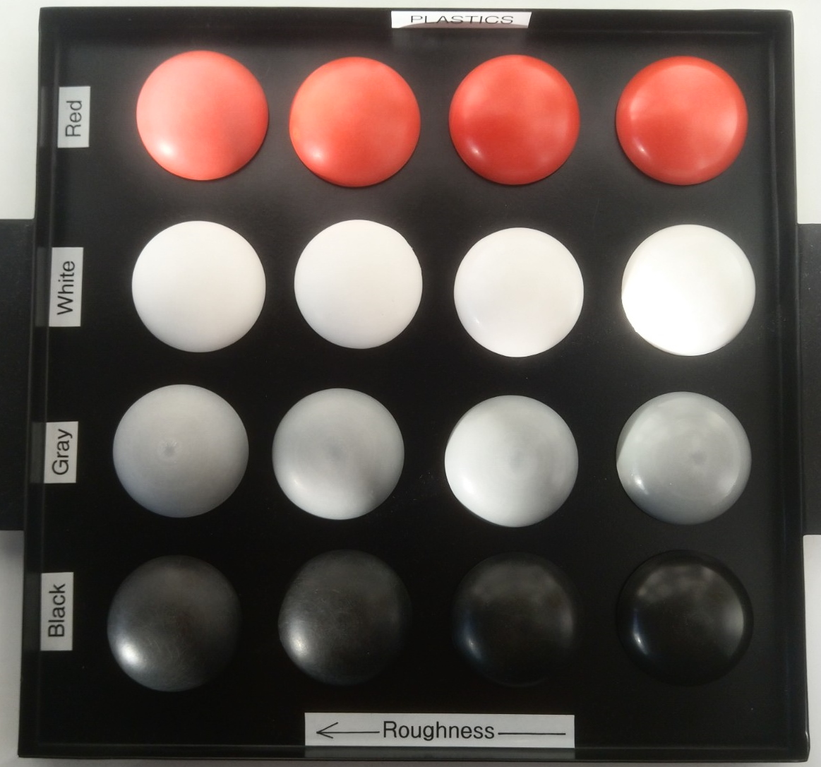
Below there are 2 trays of hemispheres of different materials. On the left you can see colored plastics and on the right are different metals.
 |
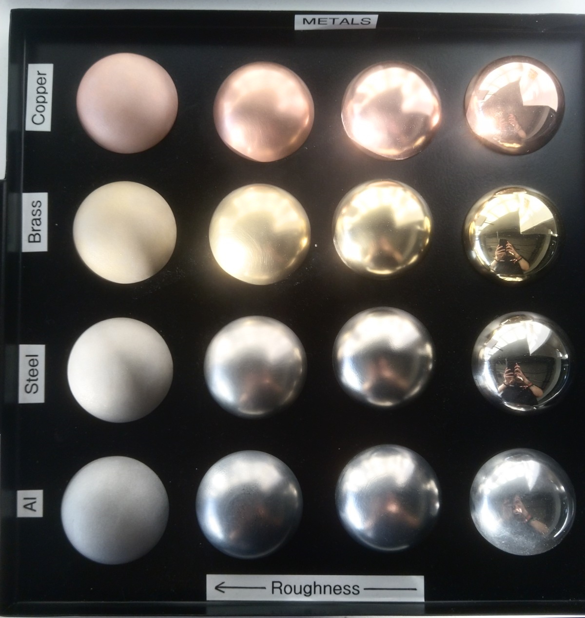 |
You can notice that even if the plastic is red, the specular highlight on it is white. This is because the color red comes from the diffuse reflectance and the highlight is the direct reflection, which comes from the specular reflection. On metals there is no diffuse reflection, only the specular, which is also tinted with the color of the metal. You can also see the sharpness of the specular reflection become more blurred to the left, when the surface roughness increases (or smoothness decreases).
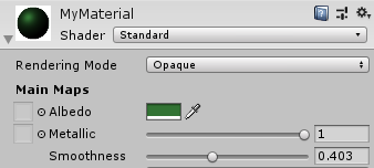
In Game Engines
Different libraries and game engines may use different formulas for actually approximating all those effects. The parameter names might be a bit different, but if it is a physically-based approach, then they try to mimic the previously described effects.
| Unreal Engine 4 | Unity |
 |
|
 |
|
| Three.js | |
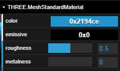 |
When using them, always read the documentation about how those parameters were meant to be used and try to understand what do they physically mean.
Links
- Real Shading in Unreal Engine 4 (2013) - Brian Karis.
How UE4 moved to PBR. - Moving Frostbite to Physically Based Rendering 3.0 (2014) - Sebastien Lagarde, Charles de Rousiers.
How the Frostbite engine moved to PBR.
* You might want to read those after/again you have gone through this topic entirely.
The Rendering Equation and BRDFs
One of the most influential formulas in computer graphics is the rendering equation. Developed by Jim Kajiya in his 1986 paper, the modern form often looks like this:
$$L_{out}(x, v) = L_{emit}(x, v) + \int_\Omega f_{brdf}(x, v, \omega_{in}) \cdot L_{in}(x, \omega_{in}) \cdot (\omega_{in} \cdot n) ~\mathrm{d} \omega_{in}$$
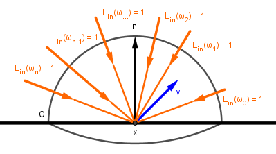
This formula describes the entire process of coloring a surface point (pixel) from a general and physically-based perspective. The formula can be read as: The outgoing light from point $x$ in the direction of $v$ is equal to the sum of two components. The first component $L_{emit}$ gives the light emitted from the surface itself at that direction. The second is the reflected (can be both diffuse and specular) light. That light is dependent on all the incoming light to that surface point. For each direction of incoming light it is the factor of the amount of incoming light $L_{in}$, how much of it is captured by a surface point at an angle ($\omega_{in} \cdot n$), how much that surface point reflects via $f_{brdf}$.
| Result | Emission | BRDF | Light Source | ||||||||||||||
| $L_{out}(x, v)$ | $=$ | $L_{emit}(x, v)$ | $+$ | $\int_\Omega$ | $f_{brdf}(x, v, \omega_{in})$ | $\cdot$ | $L_{in}(x, \omega_{in})$ | $\cdot$ | $(\omega_{in} \cdot n)$ | $~\mathrm{d} \omega_{in}$ | |||||||
 |
 |
 |
 |
 |
 |
 |
|||||||||||
| How much light is going towards the viewer from our surface point? | How much the point itself emits light? | How much light is reflected? | How much light is coming in? | How much light is captured? | |||||||||||||
| Checking all the directions on an hemisphere for incoming light. | |||||||||||||||||
Note that in the Kajiya's original paper the rendering equation was represented in terms of points. It showed how much light reaching some point from another point. This is why he also included a term for light attenuation as it travels through a medium. In other sources you might find that the rendering equation is dependent on the wavelength of light or time. There are different small variants of the equation, but the underlying meaning is always the same.
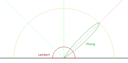
The BRDF function in this formula is the bidirectional reflectance distribution function. It returns the percentage how much of the incoming light in a given direction is reflected to another given direction at a surface point. This is the function that describes all the materials. If can represent a diffusely reflective surface, the specular reflections, metals and dielectrics etc. A good tool to visualize many common BRDF-s is the Disney's BRDF Explorer. It includes a number of common BRDF-s and you can easily add your own or modify the existing ones. It shows both in 3D and on a graph how light reflects off an object given a BRDF. For example below we have the reflection plot visualized for both Lambert and Phong BRDF-s:
There is a very good survey article by Rosana Montes and Carlos Ureña from 2012 that lists, describes and classifies a lot of the popular BRDF-s. Here is a brief redrawing of their classification with the layered BRDF class left out. The highlighted BRDF-s are the ones that we cover or discuss in this our the Computer Graphics course material.
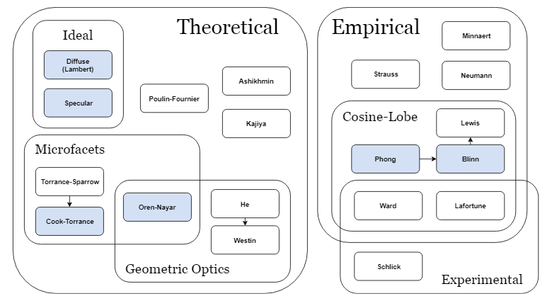
It is recommended you go check out the survey yourself and perhaps come back to that later as well.
Physically-Based Properties
Thinking about the Phong's lighting model and this rendering equation. How would the BRDF look like for that model? The most important difference you can see from the rendering equation is that the BRDF is multiplied by the $n \cdot l$. In the equation $\omega_{in}$ is the role of any given $l$ inside the integral of all possible $l$ from an hemisphere.
So if we are looking at the diffuse part of the Phong's lighting model, then the BRDF will be constant. No matter the given input vector, output vector or the surface point, we always return the same diffuse. It will basically be the diffuse color. However, if we are looking at the specular term, there is no $n \cdot l$ there. This is one reason why the Phong's lighting model is off from reality. Even for a specular highlight we need to calculate how much light is actually reaching the surface, before we reflect it. The Disney's BRDF Explorer allows you to toggle the multiplication by $n \cdot l$ when viewing a BRDF.
So you might be thinking that the Phong's lighting model can be represented as a BRDF like this:
$f = c_{diff} + c_{spec} \cdot (v \cdot r)^{shininess}$
In the reflection part of the rendering equation we would use it like:
$\color{darkgray}{\int_\Omega \color{black}{(c_{diff} + c_{spec} \cdot (v \cdot r)^{shininess})} \cdot L_{in}(x, \omega_{in}) \cdot \color{black}{(\omega_{in} \cdot n)} ~\mathrm{d} \omega_{in}}$
Notice that we are multiplying now both the diffuse and specular terms with $n \cdot l$. You are almost correct.
There are two physically-based properties we can analyze if we are interested in being more correct. These are:
- Helmholtz reciprocity principle – This is basically the bidirectionality of a BRDF. It means that the light incoming and outgoing vectors can be exchanged and the BRDF works the same way.
- Energy conservation (aka conservation of energy) – This says that there should not be any more outgoing energy than there is incoming.
Both of these properties are very important in accurate GI solutions like path tracing. You can imagine that in path tracing we are already tracing the rays from the camera, not the light source. Thus the Helmholtz reciprocity. Also because we are averaging many samples together, if there is a surface that gives out more energy than it receives, then that surface is a light source. For example if you define the emission term to be of some value. In the reflected light term it does not make sense to reflect more than was received.
To formulate the energy conservation term more easily, we can make some assumptions. Let's assume the light coming in will be $1$ regardless of the direction. Then we are interested if given an arbitrary viewer direction, we also get $1$ or less as reflected light. If it is more, then there is more energy leaving the surface than entering.
Also we disregard the emission term, because we are interested in the reflection. With these assumptions we can write the condition:
$$\int_\Omega f_{brdf}(x, v, \omega_{in}) \cdot \color{darkgray}{L_{in}(x, \omega_{in})} \cdot (\omega_{in} \cdot n) ~\mathrm{d} \omega_{in} = \int_\Omega f_{brdf}(x, v, \omega_{in}) \cdot \color{darkgray}{1} \cdot (\omega_{in} \cdot n) ~\mathrm{d} \omega_{in} = \int_\Omega f_{brdf}(x, v, \omega_{in}) \cdot (\omega_{in} \cdot n) ~\mathrm{d} \omega_{in} \leq 1$$
This condition can be analytically checked for some simpler BRDF-s. In reality there can be physically-based BRDF-s that do not satisfy it in some fringe conditions (like grazing viewer directions etc) or even ones that do not satisfy it at all, but are easy to calculate and produce visually nice results.
Energy Conservation in Lambert
We saw that the BRDF for the Lambert ideal diffuse model is just a constant term $c_{diff}$. It is the color of the material and in RGB the values can be from $0$ to $1$, right? Does it conserve energy?
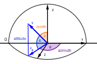
To answer that question we need to somehow collapse the integral and find out its value. For evaluating an integral over a hemisphere it is common to represent our hemisphere surface space in a spherical coordinate system. Because we are on a unit hemisphere with $r=1$, there are only two angles to consider:
- Azimuth $\phi$ – the angle on the surface plane.
- Altitude $\alpha$ – the angle on a plane perpendicular to the surface plane.
Often instead of the amplitude angle the zenith angle $\theta$ is used instead. The zenith angle is the angle between the surface normal and the corresponding vector. Here we will use the amplitude angle, but you can see how it relates to the zenith angle.
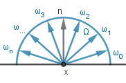
Now, integrating over the hemisphere is the same as first integrating over the altitude $\alpha$ (or zenith $\theta$) angle from $0$ to $\pi \over 2$ (half circle up) and then over the azimuth angle $\phi$ from $0$ to $pi$ (full circle around). There is one caveat there. Each full circle around the azimuth is smaller further up we get on the hemisphere. Turns out that they are $\cos(\alpha) = \sin(\theta)$ times the largest circle at the bottom, which is a unit circle because we have a unit hemisphere. So the process is like this:
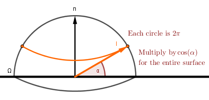
The hemisphere integral can thus be split:
$$\int_\Omega ... ~\mathrm{d} \omega = \int_{-\pi}^{\pi} \int_{0}^{\pi \over 2} ... ~ \cos(\alpha) ~\mathrm{d} \alpha ~\mathrm{d} \phi = \int_{-\pi}^{\pi} \int_{0}^{\pi \over 2} ... ~ \sin(\theta) ~\mathrm{d} \theta ~\mathrm{d} \phi$$
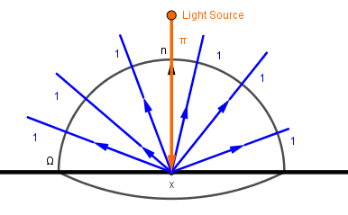
Now we can get to finding out what happens with the energy in the case of the ideal diffuse BRDF. We assume again that from every direction the amount of light coming in is $L_{in} = 1$. Let's put the maximum value $1$ as the BRDF as well. Because (like before) we assume that the surface diffusely reflects $100\%$ of the incoming light. When we put these values into the rendering equation, we get:
$$\int_\Omega 1 \cdot 1 \cdot (n \cdot \omega)... ~\mathrm{d} \omega = \int_{-\pi}^{\pi} \int_{0}^{\pi \over 2} \cos(\theta) \cdot \cos(\alpha) ~\mathrm{d} \alpha ~\mathrm{d} \phi = \int_{-\pi}^{\pi} \int_{0}^{\pi \over 2} \sin(\alpha) \cdot \cos(\alpha) ~\mathrm{d} \alpha ~\mathrm{d} \phi$$
To evaluate this, we would need the antiderivative of the $\sin(\alpha) \cdot \cos(\alpha)$. There exists a product rule of derivation, which states that: $(f(x) \cdot g(x))' = f'(x) \cdot g(x) + f(x) \cdot g'(x)$. If we put $sin(\alpha)$ in there for both $f(x)$ and $g(x)$, we get:
$$(\sin(\alpha) \cdot \sin(\alpha))' = \cos(\alpha) \cdot \sin(\alpha) + \sin(\alpha) \cdot \cos(\alpha) = 2 \cdot \sin(\alpha) \cdot \cos(\alpha)$$
This is almost what we need. To actually use this for evaluating the derivative, we need to multiply the integrand by $2$ and divide the result by $2$ afterwards (because it is a constant factor and can be brought out of the integral. Let's evaluate the inner integral first.
$$\int_{0}^{\pi \over 2} \sin(\alpha) \cdot \cos(\alpha) ~\mathrm{d} \alpha = {1 \over 2} \cdot \int_{0}^{\pi \over 2} 2 \cdot \sin(\alpha) \cdot \cos(\alpha) ~\mathrm{d} \alpha = {1 \over 2} \cdot (\sin^2(\alpha)) {\huge|}_{0}^{\pi \over 2} = {1 \over 2} \cdot \left( \sin^2(0) - \sin^2 \left( {\pi \over 2} \right) \right) = {1 \over 2} \cdot (-1) = - {1 \over 2} $$
Alright, and now let's plug this into the outer integral:
$$\int_{-\pi}^{\pi} - {1 \over 2} ~\mathrm{d} \phi = - {1 \over 2} \cdot (\phi) {\huge|}_{-\pi}^{\pi} = - {1 \over 2} \cdot (-\pi - \pi) = {2 \cdot \pi \over 2} = \pi$$
This means that if we are looking at our surface from some viewer vector $v$, then we see $\pi$ light being reflected. This is regardless of the actual $v$, so for all the different $v$ vectors we could pick from the hemisphere, we get $\pi$ light. If you think about this, then this does not make sense. There are many different $v$ vectors on the hemisphere as there are incoming light $l$ vectors. The total amount of reflected light should be the same as incoming light and we are uniformly (diffusely) reflecting it to all directions. So in our case for one direction $v$ we should get the same amount of light as is coming in at one direction $l$, which is $1$, not $\pi$.
This is why the ideal diffuse BRDF is actually $color \over \pi$.
The reason why you usually do not do this is because how light sources are defined. For analytical (point, directional, spot) light sources we define their color such that when it is full white $[1, 1, 1]$ and that light is directly shining on an ideal full white diffuse surface, then that surface should also be seen as full white [1, 1, 1] from any angle. To understand this we can just reverse the situation we had before. We replace the single viewer with a single incoming light vector and ask how much light should come in for the surface to be full white from every angle? You can reverse the situation because our BRDF follows the Helmholtz reciprocity principle. So that amount of incoming light too must be $\pi$.
With this kind of definition for our light sources, the $\pi$ in $\pi \cdot color_{light} \cdot {1 \over \pi} \cdot color_{material}$ cancels out. Do note that this definition of light sources is not actually physically correct. This also means that as soon as we do not use our analytical light sources, but instead sample the environment for incoming light, then we need to divide that light by $\pi$ if we want to use the BRDF without the $1 \over \pi$ term. Now you know how and where this term comes from.
Energy Conservation in Phong
We can derive a similar normalization term for the Phong lighting model's specular component as well. You can see the derivation in the 2009 article by Fabian Giesen. Basically if you multiply the specular term with $n \cdot l$ then you get the normalization term to be:
$$shininess + 2 \over 2 \cdot \pi$$
If you do not multiply with $n \cdot l$ as we did not in the Computer Graphics course and was not done in the original model, then you get the term to be:
$$shininess + 1 \over 2 \cdot \pi$$
Again the $\pi$ cancels out if you use analytical light sources.
On the right there is an example where the left sphere has the Phong's specular highlight as we did it before. The right sphere has the both the multiplication by $n \cdot l$ and the normalization term.
Links
- The Rendering Equation (1986) – James T. Kajiya.
The original paper of the rendering equation. - BRDF Explorer – Walt Disney Animation Studios.
Excellent tool for visualizing different BRDF-s. - An Overview of BRDF Models (2012) – Rosana Montes, Carlos Ureña.
Excellent survey article about different popular BRDF-s. - Where that #!@&?$^*%! PI comes from (2014) – Joshua Barczak.
Blogpost about the derivation of the normalization factor of diffuse BRDF-s. - PI or not to PI in game lighting equation (2012) – Sébastien Lagarde.
Blogpost about normalizing the diffuse BRDF or not. - The Blinn-Phong Normalization Zoo (2011) – Christian Schüler.
Blogpost about the different Phong and Blinn-Phong normalization terms. - Energy Conservation in Games (2009) – Rory Driscoll.
Blogpost about using the normalization terms in practice.
Microfacets
In order to model surface roughness we need a BRDF that describes also the microfacets. There is a solid theory of microfacets, which is useful to read about. Here we will try to provide the main principles in an easier way.
Basically a BRDF $f$ that accounts for microfacets can be described like this:
$$f(n, l, v) = {1 \over {(n \cdot v) \cdot (n \cdot l)}} \cdot \int_\Omega f_{\mu}(l, \omega) \cdot D(\omega) \cdot G(l, v, \omega) \cdot (\omega \cdot v) \cdot (\omega \cdot l) ~ \mathrm{d} \omega$$
The integral over $\Omega$ is over the hemisphere on the surface point that we are rendering. Just like in the Rendering Equation before. We go through all the different normal vectors on that hemisphere. For each of them we need to check:
- The percentage how much the microsurfaces with the normal $\omega$ receive incoming light – the factor $\omega \cdot l$ and final division by $n \cdot l$.
- The percentage how much the microsurfaces with the normal $\omega$ cover the pixel – the factor $\omega \cdot v$ and final division by $n \cdot v$.
- The area of the microsurface where the normals are in the direction of $\omega$ – the distribution term $D(\omega)$.
- The percentage of the microsurfaces with the normal $\omega$ that are masked and/or shadowed – the geometry term $G(l, v, \omega)$.
- The amount of light that is radiated by the microsurface itself – the microsurface's BRDF $f_{\mu}$.
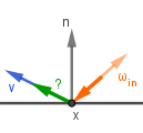
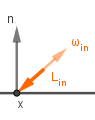
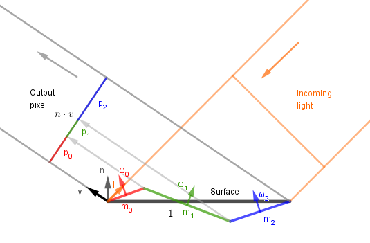
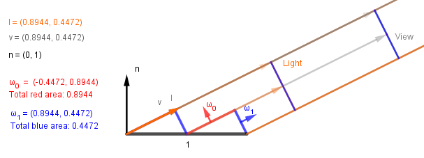
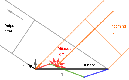
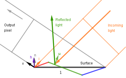
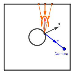
Let's look in more detail what each of those terms does. Imagine the following standard case:
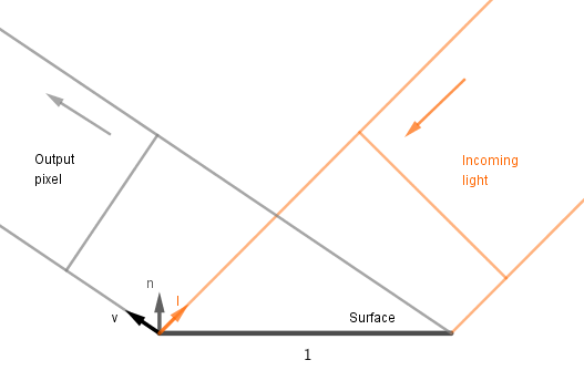
We have a unit of surface, some amount of incoming directional light, a viewer whose pixel that surface covers. Note that this unit of surface is not in any particular coordinate space, but rather just a spot we are investigating. Think about it like that we are looking at an area that is projected into a single pixel on the screen.
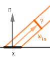
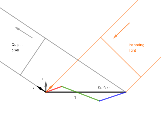
Now we are going to add microfacets (in red, green and blue). This is sub-pixel geometry that is not actually geometrically modeled, but rather we want to make the lighting work as if they were there.
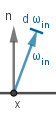
1. We want to know how much incoming light lands on each of the facets. For that we can project the facets on the plane perpendicular to the light. This is the same trick we use if we want to derive the $n \cdot l$ in Lambertian material. The cosine function is defined as a ratio of the adjacent leg to the hypotenuse in a right triangle. Note also that we are not iterating over microsurfaces, but over different microsurface normal vectors.
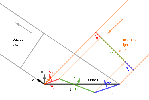
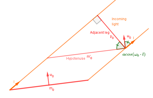
So $p_i = m_i \cdot \cos(\angle{\omega_i, l}) = m_i \cdot \omega_i \cdot l$.
Okay, but we do not know the areas ($m_i$) of the microfacets. We do not actually need to yet because currently we are looking for the percentage they make of the whole ($p_i / (p_0 + ... + p_n)$). So we need to know how much total light falls on the surface. This can be found by $n \cdot l$, as we know, which equals: $n \cdot l = p_0 + ... p_n$. That is how we can account for the light received by each microfacet. Also, the percentages found with $l \cdot \omega$ need to be signed as if the slopes are high, the microfacets could be behind each other and thus we need to account for the opposite facing facets with a negative sign.
$$\color{darkgray}{f(n, l, v) = {\color{orange}{\pmb{1}} \over {(n \cdot v) \cdot \color{orange}{\pmb{(n \cdot l)}}}} \cdot \int_\Omega f_{\mu}(l, \omega) \cdot D(\omega) \cdot G(l, v, \omega) \cdot (\omega \cdot v) \cdot \color{orange}{\pmb{(\omega \cdot l)}} ~ \mathrm{d} \omega}, ~~ \color{orange}{\pmb{-1 \leq \omega \cdot l \leq 1}}$$
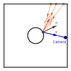
2. As each of those microfacets receives a different amount of light, it also reflects a different amount of light towards the viewer. The actual amount depends on other terms as well, but overall we can understand that it becomes important how much of each microfacet is visible to the viewer. So we need to do the same trick that we did with received light before. Just that now we are looking for the percentages of how much of each microfacet makes up the pixel.
This is where the $1 / (n \cdot v)$ and $(\omega \cdot v)$ terms come from.
$$\color{darkgray}{f(n, l, v) = {\color{teal}{\pmb{1}} \over {\color{teal}{\pmb{(n \cdot v)}} \cdot (n \cdot l)}} \cdot \int_\Omega f_{\mu}(l, \omega) \cdot D(\omega) \cdot G(l, v, \omega) \cdot \color{teal}{\pmb{(\omega \cdot v)}} \cdot (\omega \cdot l) ~ \mathrm{d} \omega}, ~~ \color{teal}{\pmb{-1 \leq \omega \cdot v \leq 1}}$$
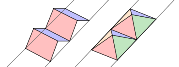
3. Next let's look at the distribution term $D(\omega)$. Previously we found the percentages of how much each microfacet is projected (towards the viewer and light). However we have no idea how big the microfacets actually are. The bigger the area, which is projected, the bigger its contribution. Imagine that you split each microfacet into a number of uniformly sized areas (or uniformly spaced points). Each of those contributes to the final projected area. On the image below there are 2 microfacets that both project to 50% of the final pixel. However, $m_0$ is twice as big as $m_1$ and light received from that is twice as much (assuming everything else is same for $m_0$ and $m_1$).
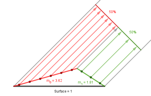
This is what the function $D(\omega)$ accounts for. It should return the total area of the microfacets that have the normal $\omega$.
$$\color{darkgray}{f(n, l, v) = {1 \over {(n \cdot v) \cdot (n \cdot l)}} \cdot \int_\Omega f_{\mu}(l, \omega) \cdot \color{blue}{\pmb{D(\omega)}} \cdot G(l, v, \omega) \cdot (\omega \cdot v) \cdot (\omega \cdot l) ~ \mathrm{d} \omega}, ~~ \color{blue}{\pmb{0 \leq D(\omega) < \infty}}$$
4. The geometry term $G(l, v, \omega)$ deals with shadowing and masking. The microfacets can shadow each other from incoming light or mask each other from the view.
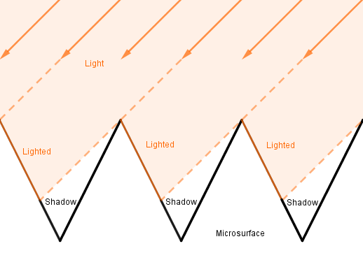
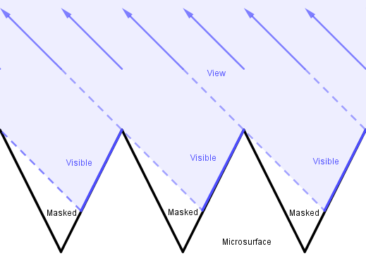
The function $G(l, v, \omega)$ should give a percentage how much of the microfacets with the given normal are not masked or shadowed given view and light vectors. Notice that with the V-cavities above if the view and light vectors are on the same side of a microfacet, then we care about the maximum of either visible or lighted percentage. If the view and light are on the opposite sides and a face is either masked or shadowed, it is so fully, so again the maximum value is the one we want.
$$\color{darkgray}{f(n, l, v) = {1 \over {(n \cdot v) \cdot (n \cdot l)}} \cdot \int_\Omega f_{\mu}(l, \omega) \cdot D(\omega) \cdot \color{green}{\pmb{G(l, v, \omega)}} \cdot (\omega \cdot v) \cdot (\omega \cdot l) ~ \mathrm{d} \omega}, ~~ \color{green}{\pmb{0 \leq G(l, v, \omega) \leq 1}}$$
The geometry term is usually quite dependent on the actual shapes of the microfacets. So for an accurate geometry term one would have to know how the microfacets are laid out. Just the distribution term does not give that as there can be different configurations with the same distribution of normals, but with different geometry.
5. Lastly we have the BRDF of the microfacet itself. Usually we can assume that the microfacets themselves are either perfect diffuse or specular reflectors. So Lambert or a perfect mirror, depending on which surface we are modelling.
6*. There is actually one more effect sometimes considered. That is the interreflection of light between the microfacets.
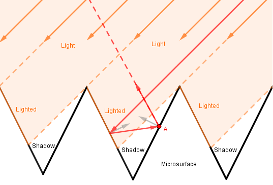
Here the point $A$ would otherwise be in shadow, but because light can reflect off the opposite microfacet, then in reality it does contribute to the result. Modelling this effect can be complicated.
Example
Let's now see how our microfacet formula works under certain conditions. We are interested in the final illumination value, so we can replace it into the rendering equation.
$$L_{out} = L_{emit} + \int_\Omega \left ( {1 \over {(n \cdot v) \cdot (n \cdot l)}} \cdot \int_\Omega f_{\mu}(l, \omega) \cdot D(\omega) \cdot G(l, v, \omega) \cdot (\omega \cdot v) \cdot (\omega \cdot l) ~ \mathrm{d} \omega \right ) \cdot L_{in}(\omega) \cdot n \cdot l ~ \mathrm{d} \omega$$
Notice that the term $n \cdot l$ cancels out from our microfacet BRDF and the rendering equation.
$$L_{out} = L_{emit} + \int_\Omega \left ( {1 \over {(n \cdot v) \cdot \color{orange}{\pmb{(n \cdot l)}}}} \cdot \int_\Omega f_{\mu}(l, \omega) \cdot D(\omega) \cdot G(l, v, \omega) \cdot (\omega \cdot v) \cdot (\omega \cdot l) ~ \mathrm{d} \omega \right ) \cdot L_{in}(\omega) \cdot \color{orange}{\pmb{n \cdot l}} ~ \mathrm{d} \omega$$
Let's also simplify this. Assume our material does not emit any light. Also that we have a single directional light source and we do not care about light bounces in the scene. That assumption will allow us to remove the outer integral as $L_{in}({\omega})$ will be 0 anywhere but at our light direction.
$$L_{out} = \left ( {1 \over {(n \cdot v)}} \cdot \int_\Omega f_{\mu}(l, \omega) \cdot D(\omega) \cdot G(l, v, \omega) \cdot (\omega \cdot v) \cdot (\omega \cdot l) ~ \mathrm{d} \omega \right ) \cdot L_{in}(l) $$
Assume our light is shining at full intensity, so $L_{in}(l) = 1$, and remove that term.
$$L_{out} = {1 \over {(n \cdot v)}} \cdot \int_\Omega f_{\mu}(l, \omega) \cdot D(\omega) \cdot G(l, v, \omega) \cdot (\omega \cdot v) \cdot (\omega \cdot l) ~ \mathrm{d} \omega $$
Lastly we discard the geometry term (do not account for shadowing and masking). The geometry term would affect the result at grazing angles.
$$L_{out} = {1 \over {(n \cdot v)}} \cdot \int_\Omega f_{\mu}(l, \omega) \cdot D(\omega) \cdot (\omega \cdot v) \cdot (\omega \cdot l) ~ \mathrm{d} \omega $$
Next we should define our microsurface. We want to specify our geometry. Let's assume we have some V-cavities that are symmetric in one direction only. This allows us to play through the example by only looking at a hemicircle instead of a hemisphere. You can think about how this would play out in 3D.
Our simple V-cavity will look from the side like this:
Now we need our distribution function $D(\omega)$ to mathematically represent this. Because there are only 2 microsurface directions we need $D(\omega)$ to output the area values at locations $\omega_0$ and $\omega_1$ and be 0 everywhere else. This can be done using a Dirac delta function $\delta$. It is a construct that has 0 everywhere except at a point $p$ ($p=0$ by default), where it is $\infty$.
$\begin{align*} &\delta(x, p = 0) = \begin{cases} \infty, & \text{if } x = p \\ 0 \end{cases} \end{align*} $
It also integrates to value 1 and if it is multiplied with some other function of $x$, then the integral is that function at $p$.
$\int \delta(x) ~ \mathrm{d} x = 1 $
$\int f(x) \cdot \delta(x, p) ~ \mathrm{d} x = f(p) $
Now we can define the distribution term as:
$$D(\omega) = \color{red}{\delta(\omega, \omega_0) \cdot m_0} + \color{blue}{\delta(\omega, \omega_1) \cdot m_1},$$
where the $\color{red}{m_0}$ and $\color{blue}{m_1}$ are the respective microsurface areas.
Let's denote everything else we have under the integral in the microfacet formula as $\color{darkgray}{other(\omega)}$. Then we get:
$$L_{out} = {1 \over {(n \cdot v)}} \cdot \int_\Omega D(\omega) \cdot \color{darkgray}{other(\omega)} ~ \mathrm{d}\omega $$
$$L_{out} = {1 \over {(n \cdot v)}} \cdot \int_\Omega (\color{red}{\delta(\omega, \omega_0) \cdot m_0} + \color{blue}{\delta(\omega, \omega_1) \cdot m_1}) \cdot \color{darkgray}{other(\omega)} ~ \mathrm{d}\omega $$
$$L_{out} = {1 \over {(n \cdot v)}} \cdot \int_\Omega \color{red}{\delta(\omega, \omega_0) \cdot m_0} \cdot \color{darkgray}{other(\omega)} + \color{blue}{\delta(\omega, \omega_1) \cdot m_1} \cdot \color{darkgray}{other(\omega)} ~ \mathrm{d}\omega $$
The integral of a sum is the sum of integrals of the addends.
$$L_{out} = {1 \over {(n \cdot v)}} \cdot \left (\int_\Omega \color{red}{\delta(\omega, \omega_0) \cdot m_0} \cdot m_0 \cdot \color{darkgray}{other(\omega)} ~ \mathrm{d}\omega + \int_\Omega \color{blue}{\delta(\omega, \omega_1) \cdot m_1} \cdot \color{darkgray}{other(\omega)} ~ \mathrm{d}\omega \right ) $$
The $\color{red}{m_0}$ and $\color{blue}{m_1}$ are constant terms and this means that we can evaluate our surface with just a sum*:
$$L_{out} = {1 \over {(n \cdot v)}} \cdot (\color{red}{m_0} \cdot \color{darkgray}{other(\color{red}{\omega_0})} + \color{blue}{m_1}\cdot \color{darkgray}{other(\color{blue}{\omega_1})}) $$
* Note that we actually did the same thing implicitly when we got rid of all the incoming light directions in favor of one in the rendering equation before.
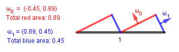
Nice, this means that we can easily evaluate what happens on our specific microsurface if we fix some light and view directions. So let's do that. Consider this case:
Plugging in the numbers we get:
| $\omega$ | $m$ | $\omega \cdot v$ | $\omega \cdot l$ | product | division by $n \cdot v$ |
| $\omega_0 = (-0.45, 0.89)$ | $0.89$ | $0.96$ | $0.55$ | $0.47$ | $0.48$ |
| $\omega_1 = (0.89, 0.45)$ | $0.45$ | $0.29$ | $0.83$ | $0.11$ | $0.11$ |
| Result: | $0.59$ | ||||
So the intensity of light reflected off that microsurface to the viewer is $0.59$ (59%). Without the microsurface, if we would just apply Lambert, we get $n \cdot l = 0.866$ (87%).
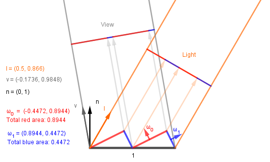
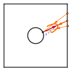
Let's also look at another case, where the light and view directions are the same and perpendicular to the blue microfacet:
Here we get:
| $\omega$ | $m$ | $\omega \cdot v$ | $\omega \cdot l$ | product | division by $n \cdot v$ |
| $\omega_0 = (-0.45, 0.89)$ | $0.89$ | $0.00$ | $0.00$ | $0.00$ | $0.0$ |
| $\omega_1 = (0.89, 0.45)$ | $0.45$ | $1.00$ | $1.00$ | $0.45$ | $1.00$ |
| Result: | $1.00$ | ||||
We get the full intensity 100% back as expected. This makes sense because the light and viewer are perpendicular to the microfacets that cover the projection plane. If we would just apply Lambert, we would get 45% intensity at that angle.
Now we have seen how microfacets affect the light calculations. In our example we had one very specific surface and we managed to calculate the final intensity values. In reality you would want to be able to control the angles of the microfacets and have a better distribution of them. In surfaces there are many microfacets under different angles, so a controllable distribution would account for that. In that case you would not be able to use the Dirac delta function and get a small finite number of terms. Instead when people come up with formulae to satisfy the microfacet formula, they then try to solve the integral analytically to find one formula that gives the result without having to integrate. If such closed-form equation is not possible or feasible because of the complexity of the integral, then different numerical approximations to it can be applied.
Links
- Understanding the Masking-Shadowing Function in Microfacet-Based BRDFs (2014) - Eric Heitz.
Thorough and very insightful coverage of the microfacet theory with a lot of good references. - Microfacet Models for Refraction through Rough Surfaces (2007) - Walter et al.
The derivation of GGX BRDF, but the microfacet theory chapter (3) gives a good and concise description. - Microfacet BRDF (2011) - Simon's Tech Blog.
Some description of different distribution and geometry terms with refs and a live example.
Oren-Nayar
In 1994 M. Oren and S. K. Nayar found out that the ever-popular Lambertian diffuse model is accurate only for totally smooth surfaces. However, most surfaces have some kind of roughness, which can be described as microfacets. In their paper Oren and Nayar describe how that roughness affects the reflectance properties of materials. As the authors come from the field of computer vision, the derivation of the model uses a bit different notation. But they do describe the V-shaped microfacets (V-cavities), shadowing, masking and interreflections. They then build 3 different models that build on each other: isotropic single-slope, gaussian-slope and qualitative. Each uses Lambertian (ideal diffuse) microfacets.
All the models use V-cavities and the gaussian-slope one uses a Gaussian distribution to vary the surface roughness. Like we thought before, the surfaces should have different facets with varying slope. Gaussian distribution of the slope seems like the way to model this effect. The roughness value there is the standard deviation $\sigma$ of the distribution. The more rough the surface is, more higher slope facets should there be. The mean $\mu$ is always the direction perpendicular to the surface. So when the roughness is 0, we have a flat surface and the model is equivalent to Lambert. The difference is visualized on the example to the right. There the left material is pure Lambertian surface and the right one uses the gaussian-slope Oren-Nayar BRDF. You can notice that the more rough the surface is, the more flat it will visually appear. This effect was confirmed with different examples of real life surfaces (most prominently with the vase) in the paper.
When you check the formula from the paper you can see that it is quite involved and uses polar angles instead of vectors like we are used to. Furthermore, their integral did not have a closed form, so they numerically approximated it. That is why there is also the third qualitative model:
$$f_{orenNayar}(\theta_v,~ \theta_l,~ \phi_v - \phi_l,~ \sigma) = {{\rho} \over {\pi}} (A + B \cdot \max(0,~ \cos(\phi_v - \phi_l)) \cdot \sin(\alpha) \cdot tan(\beta))$$
where:
$A = 1.0 - 0.5 {{\sigma^2} \over {\sigma^2 + 0.33}}$
$B = 0.45 {{\sigma^2} \over {\sigma^2 + 0.09}}$
$\alpha = \max(\theta_v,~ \theta_l) ~~~~~ \beta = \min(\theta_v,~ \theta_l)$
The term ${{\rho} \over {\pi}}$ is the Lambertian BRDF. The division by $\pi$ is because of the energy conservation as explained in the BRDF section and thus depends on your implementation. The $\rho$ is the color of the surface. The standard deviation $\sigma$ represents the roughness of the surface.
As we can see, the formula depends on the zenith ($\theta$) and azimuth ($\phi$) angles of our vectors ($v$ for view and $l$ for light). These are tedious and wasteful to calculate on the GPU. Thus J. van Ouwerkerk has come up with a rewrite of the formula in 2011.
1) We can represent the $\sin$ and $\tan$ functions via the $\cos$ function. Namely:
$\sin(\alpha) = \sqrt{1 - \cos^2(\alpha)}$
$\tan(\beta) = {\sin(\beta) \over \cos(\beta)} = {\sqrt{1 - \cos^2(\beta)} \over \cos(\beta)} $
Substituting these will get us:
$$\color{darkgray}{f_{orenNayar}(\theta_v,~ \theta_l,~ \phi_v - \phi_l,~ \sigma) = {{\rho} \over {\pi}} \cdot \left ( A + B \cdot \max(0,~ \cos(\phi_v - \phi_l)) \cdot \color{black}{\sqrt{1 - \cos^2(\alpha)} \cdot{\sqrt{1 - \cos^2(\beta)} \over \cos(\beta)}} \right )}$$
$$\color{darkgray}{f_{orenNayar}(\theta_v,~ \theta_l,~ \phi_v - \phi_l,~ \sigma) = {{\rho} \over {\pi}} \cdot \left ( A + B \cdot \max(0,~ \cos(\phi_v - \phi_l)) \cdot \color{black}{{{\sqrt{(1 - \cos^2(\alpha)) \cdot (1 - \cos^2(\beta))}} \over {\cos(\beta)}}} \right )}$$
2) Now we can see that in the numerator $\alpha$ and $\beta$ are interchangeable. So we do not need to take both $\max$ and $\min$ for the $\alpha$ and $\beta$, but it only suffices to find the $\beta = \min(\theta_l, \theta_v)$.
$$\color{darkgray}{f_{orenNayar}(\theta_v,~ \theta_l,~ \phi_v - \phi_l,~ \sigma) = {{\rho} \over {\pi}} \cdot \left ( A + B \cdot \max(0,~ \cos(\phi_v - \phi_l)) \cdot \color{black}{{{\sqrt{(1 - \cos^2(\theta_l)) \cdot (1 - \cos^2(\theta_v))}} \over {\cos(\min(\theta_l,~ \theta_v))}}} \right )}$$
3) We would like to get rid of the angles in favor of their cosines. So let's look how the cosine function behaves:
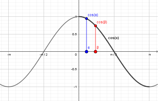
Our zenith angles are from $[0, \pi]$ and the cosine function is continuously decreasing on that range. This means that we can substitute the minimum on the angles with the maximum of their cosines.
$\cos(\min(\theta_l, \theta_v)) = \max(\cos(\theta_l), \cos(\theta_v))$
As we were taking the cosine of the angle anyway afterwards, the maximum cosine will be in the denominator.
$$\color{darkgray}{f_{orenNayar}(\theta_v,~ \theta_l,~ \phi_v - \phi_l,~ \sigma) = {{\rho} \over {\pi}} \cdot \left ( A + B \cdot \max(0,~ \cos(\phi_v - \phi_l)) \cdot {{\sqrt{(1 - \cos^2(\theta_l)) \cdot (1 - \cos^2(\theta_v))}} \over \color{black}{{\max(\cos(\theta_l),~ \cos(\theta_v))}}} \right )}$$
4) Unfortunately we can not do anything better with the azimuth angles besides projecting the vectors down to the surface plane and taking their dot product there.
$v_{proj} = \mathrm{normalize}(v - n \cdot \max(0,~ (n \cdot v)))$
$l_{proj} = \mathrm{normalize}(l - n \cdot \max(0,~ (n \cdot l)))$
These projections just find the component parallel to the surface normal and subtract it from the vectors.
$$\color{darkgray}{f_{orenNayar}(\theta_v,~ \theta_l,~ \phi_v - \phi_l,~ \sigma) = {{\rho} \over {\pi}} \cdot \left ( A + B \cdot \color{black}{\max(0,~ v_{proj} \cdot l_{proj})} \cdot {{\sqrt{(1 - \cos^2(\theta_l)) \cdot (1 - \cos^2(\theta_v))}} \over {\max(\cos(\theta_l),~ \cos(\theta_v))}} \right )}$$
5) Fortunately we now have just two cosines we can reuse.
$L = \max(0,~ l \cdot n)$
$V = \max(0,~ v \cdot n)$
$v_{proj} = normalize(v - n \cdot V)$
$l_{proj} = normalize(l - n \cdot L)$
Thus the final form of the rewritten formula is:
$$f_{orenNayar}(\theta_v,~ \theta_l,~ \phi_v - \phi_l,~ \sigma) = {{\rho} \over {\pi}} \cdot \left ( A + B \cdot \max(0,~ v_{proj} \cdot l_{proj}) \cdot {{\sqrt{(1 - L^2) \cdot (1 - V^2)}} \over {\max(L,~ V)}} \right )$$
This one uses only the dot products between the vectors like we are used to in computer graphics. It does have one square root, which can be considered a problem.
Visually the qualitative model is also different from the full Oren-Nayar model. Several terms were removed. This causes noticeable dark rings to appears on the objects, because $C^1$ smoothness violations. Somewhere around 2013 Y. Fujii came up with an improved Oren-Nayar model that is of $C^2$ smoothness and is (at the time of writing) used in Blender modelling software. The improvement uses also only vector math and does not include the square root.
On the example to the right the left material is the qualitative model implemented via the Ouwerkerk's rewrite and the right one is the improved Oren-Nayar model. If you make the surface rough and move the light source, you should be able to see a dark ring appearing on the surface with the qualitative model.
Using the Disney's BRDF explorer we can also compare each of the functions. With $\theta_l \approx 24°$ and $\theta_v \approx 57°$:
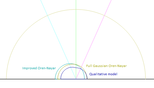
You can see the 1st order discontinuity in the blue qualitative model, which causes the dark circle.
One can wonder if the improved Oren-Nayar and the qualitative model are still physically-based or have they been too much approximated and mathematically improved to be considered such.
Links
- Generalization of Lambert’s Reflectance Model (1994) - Michael Oren and Shree K. Nayar.
The original paper deriving the Oren-Nayar reflectance model. - Van Ouwerkerk's rewrite (of the Oren Nayar BRDF) (2011) - Jos van Ouwerkerk.
Rewrite of the Oren-Nayar model for better use in computer graphics. - A Tiny Improvement of Oren-Nayar Reflectance Model (~2013) - Yasuhiro Fujii.
Improved version of the qualitative Oren-Nayar model with $C^2$ smoothness.
Fresnel Effect
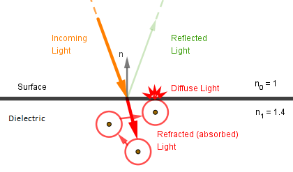
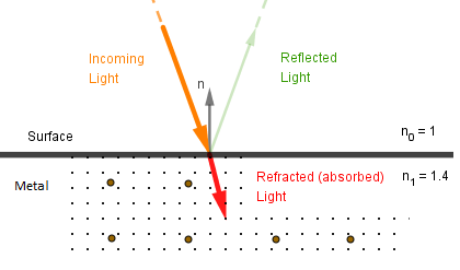
The amount of light that is either reflected or absorbed by the material depends on the angle the light is coming at the surface (angle of incidence). This is true for all materials, be it metal or dielectric. This effect that the material reflects a different amount of light depending on the angle of incidence is called the Fresnel effect.
If the angle of incidence is small, the incoming light is more perpendicular to the surface. This means that more of the light penetrates the surface. If the surface is opaque, that light is absorbed. In case of dielectrics, the energy absorbed travels through the atoms and exits the surface at some other angle as diffuse light. In the case of metals it is absorbed into the electron gas.
This is what we also learned in the Metals and Dielectrics chapter. However, if the angle of incidence is larger, more light gets directly reflected off the surface.
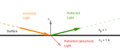
So if the light is shining at a surface at grazing angles, we should see more specular reflection of the light. Or if we are looking at the surface at grazing angles, we should see more of the environment reflected off the surface.
We see this effect every day. The common example is water. If you are on the beach and standing in the water and looking straight down, you usually do not see your own reflection. However, if it is now evening and the sun is setting, you will see the reflection of the sun on the distant sea. Just like you see the reflections of distant buildings or trees on the sea at any time of the day. The caveat with this example is that if the water is deep enough, you do see your own reflection even straight down. With shallow water the seabed is more illuminated and noticeable than your reflection.
[TODO real life picture?]
Different materials have a property called index of refraction. If light moves through the material with the index of refraction $n_0$ and encounters on its path some other material with index $n_1$, then the Fresnel effect occurs. Some of the light enters the new material and some reflects. How much exactly depends on the values $n_0$ and $n_1$ as well as the angle of incidence, like we just saw. You can kind of think about it like light is a bullet and the index of refraction is the hardness of the material. If you shoot your bullet at a perpendicular angle, it is more likely to penetrate the surface. If you shoot at a grazing angle, it is more likely to ricochet off. This also depends on how hard the material is, ie how much work is needed to penetrate the material.
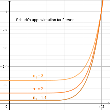
In computer graphics we use the Schlick's approximation to the actual Fresnel equations.
$R_0 = \left ({{n_0 - n_1} \over {n_0 + n_1}} \right)^2$
$F(n, l) = R_0 + (1 - R_0) \cdot (1 - n \cdot l)^5$
You can see that $R_0$ is the reflectance factor perpendicular to the surface (eg when looking straight down). If the angle of incidence becomes $90°$, the reflectance becomes $1$. So all materials become more mirror-like at more grazing angles.
Now, there are actually different values for $n$ depending on the wavelength of light. Usually values for only certain light are known. So instead of thinking about the index of refraction, we can instead think about $R_0$. You see, usually in computer graphics our light travels through air ($n_0 = 1$) and we are interested in the Fresnel effect at some certain material. This means we can think about how much that material should reflect when we are looking perpendicular to it from air. It is easier to think in those terms.
As the electron gas in metals still absorbs certain wavelengths of light for specular reflection, we have to consider color for the Fresnel effect in metals. For that we can define $R_0$ as an RGB vector. So we calculate the effect for all three color channels. However, in dielectrics the specular reflection in the different channels is usually same, so we define some small value for it. For simplicity it is usually recommend to have a single value $R_0 \in [0.01, 0.05]$ for dielectrics.
If we have $R_0 = 0.05$, we can backtrack:
$R_0 = \left ({{n_0 - n_1} \over {n_0 + n_1}} \right)^2 = 0.05 ~~~ | \sqrt{~} $
The $\sqrt{~}$ can be both positive or negative. We take the negative value.
$ {{n_0 - n_1} \over {n_0 + n_1}} \approx -0.2236 $
We are looking interaction from air to dielectric, so $n_0 = 1$ for air.
$ {{1 - n_1} \over {1 + n_1}} = -0.2236 $
$ -0.2236 - 0.2236 \cdot n_1 = 1 - n_1 $
$ 0.7764 \cdot n_1 = 1.2236 $
$ n_1 \approx 1.58 $
The refractive index for polystyrene (one of the more common plastics, eg yogurt cups are made of it) is $1.59$, which is almost what we got.
| $R_0$ | $0.01$ | $0.02$ | $0.03$ | $0.04$ | $0.05$ |
|---|---|---|---|---|---|
| $~n_1$ | $1.22$ | $1.33$ | $1.42$ | $1.5$ | $1.56$ |
| Material | - | Water, ice | Human liver | Plexiglas | Plastic, amber |
It is quite difficult to find the index of refraction for some given material. But if we now think in terms of $R_0$ we can instead define something like this:
| Material | Dielectric | Skin | Gold | Aluminimum | Copper | Iron |
| $R_0$ specular color |
$\color{white}{\small{[0.036, 0.036, 0.036]}}$ | $\color{white}{\small{[0.024, 0.024, 0.024]}}$ | $\color{black}{\small{[1.000, 0.767, 0.334]}}$ | $\color{black}{\small{[0.916, 0.924, 0.924]}}$ | $\color{black}{\small{[0.957, 0.639, 0.536]}}$ | $\color{black}{\small{[0.560, 0.580, 0.580]}}$ |
|---|
This makes more sense. We define the specular color for metals that what we think of as their color. For dielectrics we define the specular color as the percentage they should reflect when looking perpendicularly at them.
To put it all together. Opaque materials reflect and absorb (refract) different amount of light. The Fresnel effect calculated via the Schlick's approximation gives us the percentage of reflected light. Let's call that amount $\color{green}{k_{spec}} = F(n, v)$. For metals that is all there is, because everything else gets absorbed. For dielectrics rest of the light will diffusely scatter from the surface. Let's call that amount $\color{red}{k_{diff}} = 1.0 - F(n ,v) = 1.0 - \color{green}{k_{spec}}$. Lastly we need to specify if the material is a metal or not. As mentioned before, it is often defined as a continuous variable called metallic. The only thing it affects is that refracted light must get absorbed and does not come back out from the surface. So $\color{red}{k_{diff}} = (1.0 - \color{green}{k_{spec}}) \cdot (1.0 - metallic)$.
In terms of the rendering equation it would be like this:
$\color{darkgray}{\int_\Omega L(\omega_i) \cdot (n \cdot l) \cdot \color{black}{f_{brdf}} ~ \mathrm{d}\omega_i}$
$\color{darkgray}{\int_\Omega L(\omega_i) \cdot (n \cdot l) \cdot (\color{black}{\color{red}{k_{diff}} \cdot f_{diff} + \color{green}{k_{spec}} \cdot f_{spec}}) ~ \mathrm{d}\omega_i}$
$\color{darkgray}{\int_\Omega L(\omega_i) \cdot (n \cdot l) \cdot (\color{black}{\color{red}{(1.0 -F) \cdot (1.0 - metallic)} \cdot f_{diff} + \color{green}{F} \cdot f_{spec}}) ~ \mathrm{d}\omega_i}$
On the example to the right the metallic parameter is called $m$. The value $n_1$ is left in only for dielectrics. In a real application it would be replaced by a constant $R_0$ for dielectrics. The left object has only the Fresnel effect visualized. The right one multiplies it by $n \cdot l$ as well. You can check out that:
- When you set a color and then change the metallic value, the specular color goes from the defined color to a grayscale value found via $n_1$.
- The grazing angles of the material go to 1 no matter if it is metallic or not.
- When $n_1=1$ the grazing angles of the material still need to go to 1.
- When $n_1=0$ the Fresnel effect becomes 100% everywhere.
Links
- Unity's Material Charts
Reference values for different materials in the Unity game engine. - DONTNOD Physically based rendering chart for Unreal Engine 4 (2014) - Sébastien Lagarde.
Reference values for different materials in the UE4 game engine as defined by DONTNOD game dev company. - Everything has Fresnel (2010) - John Hable.
Real-life examples of materials with Fresnel. - The Comprehensive PBR Guide by Allegorithmic - vol. 1 - Wes McDermott.
Concise overview of important things PBR, including Fresnel.
Cook-Torrance
In their 1982 paper Robert L. Cook and Kenneth E. Torrance put together a specular reflectance microfacet BRDF. Differently from the Oren-Nayar model they modeled the microfacets as ideal specular reflectors (vs ideal diffuse reflectors).
 |
 |
| Ideal diffuse microfacets (Oren-Nayar) | Ideal specular microfacets (Cook-Torrance) |
|---|
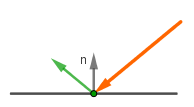
They also used V-cavities, so their geometry function $\color{green}{G}$ was the same as in Oren-Nayar. Although instead of the microsurface normal, they used the half-angle vector. This brings us to the key difference. When we use ideal specular reflectors, they are visible only when their surface normal $\omega$ is equal to the half-angle vector $\color{purple}{h}$. You might remember the Blinn-Phong model from the main Computer Graphics course, where the specular highlight was based on $n \cdot h$. If the half-angle vector between the light $l$ and viewer $v$ vectors becomes the surface normal, then the light's incident and viewer angles are the same. So the light directly reflects towards the viewer. This means that we are no longer interested in how much the microfacet normal deviates from the surface normal, instead we are interested in how much it deviates from the half-angle vector.
This brings us to the distribution term $\color{blue}{D}$. Cook and Torrance used the Beckmann distribution to find the area of the microfacet surface that is aligned with the half-angle vector:
$$D = {1 \over {m^2 \cdot (n \cdot \color{purple}{h})^4}} \cdot e^{\Large{- \left( \tan(\angle n, \color{purple}{h}) \over m \right)^2}}$$
The $\tan$ function can be easily converted to dot products (cosines):
$$D = {1 \over {m^2 \cdot (n \cdot \color{purple}{h})^4}} \cdot e^{\Large{- \left( \sqrt{1 - (n \cdot \color{purple}{h})^2)} \over (n \cdot \color{purple}{h}) \cdot m \right)^2}}$$
Now, the main contribution attributed to Cook and Torrance from that model was the form of the microfacet-based BRDF formula. Previously we derived the following formula:
$$f(n, l, v) = {1 \over {(n \cdot v) \cdot (n \cdot l)}} \cdot \int_\Omega f_{\mu}(l, \omega) \cdot D(\omega) \cdot G(l, v, \omega) \cdot (\omega \cdot v) \cdot (\omega \cdot l) ~ \mathrm{d} \omega$$
The $\int_\Omega$ here is over the hemisphere. We can think of it to follow the light vector (or viewer, or normal) across the surface of the hemisphere.
However, now that we have ideal specular reflectors as our microfacets, we want define our one microfacet BRDF to be something like:
$$f_{\mu}(l, \omega) = \delta(\omega, h)$$
So that when the given microsurface normal is equal to the half-angle vector between light and viewer, we get a response. Otherwise we get 0. Unfortunately the possible half-angle vectors are not distributed across the surface of the hemisphere the same way as $n$, $l$ or $v$ were. This means that to use that delta function as the ideal reflector, we need to normalize it. For that let's look at how the half-angle vector would cover the hemisphere, when (for example) the light vector moves. We leave the viewer vector at $0$, because we want the half-angle vector to trace the same path as $l$ in the previous example.
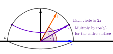
There are two things to notice here that are different from the previous integral:
- Our light vector $l$ goes twice as far for the half-angle vector $h$ to cover the full sphere. So $2 \cdot \chi = \lambda = \alpha$.
- The half-angle vector $h$ is moving twice as slow as the previous light vector: $2 \cdot \mathrm{d} \chi = \mathrm{d} \alpha$.
The process of integrating over half-angle here is different. The angle and its change is less than before. This means that we can not just replace this process in the formula, but need to normalize it first. Let's see what happens when we integrate over identity. Note that because the integral of $\cos$ is the same as integral of $\sin$ in our range from $0$ to $\pi \over 2$, we can replace the cosine with sine.
The previous process of integrating the sphere: $\int_\Omega 1 ~ \mathrm{d} \alpha = \int_{-\pi}^\pi \int_0^{\pi \over 2} 1 \cdot \cos(\alpha) ~ \mathrm{d} \alpha = \int_{-\pi}^\pi \int_0^{\pi \over 2} 1 \cdot \sin(\alpha) ~ \mathrm{d} \alpha$
The new one with half-angle vector: $\int_\Omega 1 ~ \mathrm{d} \chi = \int_{-\pi}^\pi \int_0^{\pi \over 2} 1 \cdot \cos(\chi) ~ \mathrm{d} \chi = \int_{-\pi}^\pi \int_0^{\pi \over 2} 1 \cdot \sin(\chi) ~ \mathrm{d} \chi$
We need the new one to have the same output magnitude as the previous one, so we must find the percentage of the new one to the old one and multiply it by that. We'll look at the terms under the integral to find the normalization factor:
$${{\sin(\chi) ~ \mathrm{d} \chi} \over {\sin(\alpha) ~ \mathrm{d} \alpha}} = {{\sin(\chi) ~ \mathrm{d} \chi} \over {\sin(2 \cdot \chi) ~ 2 \cdot \mathrm{d} \chi}} = {{\sin(\chi) ~ \mathrm{d} \chi} \over {2 \cdot 2 \cdot \cos(\chi) \cdot \sin(\chi) ~ \mathrm{d} \chi}} = {{1} \over {4 \cdot \cos(\chi)}}$$
One last problem is that generally a BRDF tells how much light is reflected and distributed towards different viewer vectors and how much is absorbed. Because we want to have ideal specular reflectors, we need to send the full incoming light always towards the viewer. Even if the viewer angle is small, still full incoming light is reflected, because none of it is either absorbed or goes anywhere else. So we need to also normalize with another cosine of the angle $\chi$ between the half-angle and viewer vectors. So our ideal specular microfacet BRDF will be:
$$f_{\mu}(l, \omega) = \delta(\omega, h) \cdot {1 \over {\cos(\chi)}} \cdot {1 \over {4 \cdot \cos(\chi)}} = {{\delta(\omega, h)} \over {4 \cdot \cos(\chi) \cdot \cos(\chi)}}$$
Now, on our actual surface we have a situation like this:
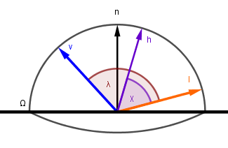
This means we can replace the cosines with dot products and finally get the ideal specular one microfacet BRDF as:
$$f_{\mu}(l, \omega) = {{\delta(\omega, h)} \over {4 \cdot \cos(\chi) \cdot \cos(\chi)}} = {{\delta(\omega, h)} \over {4 \cdot (h \cdot v) \cdot (h \cdot l)}}$$
When we insert this into our general microfacet BRDF formula we get:
$$f(n, l, v) = {1 \over {(n \cdot v) \cdot (n \cdot l)}} \cdot \int_\Omega {{\delta(\omega, h)} \over {4 \cdot (h \cdot v) \cdot (h \cdot l)}} \cdot D(\omega) \cdot G(l, v, \omega) \cdot (\omega \cdot v) \cdot (\omega \cdot l) ~ \mathrm{d} \omega$$
Now we can get rid of the integral by replacing all the $\omega = h$, because of the correctly normalized delta function.
$$f(n, l, v) = {1 \over {(n \cdot v) \cdot (n \cdot l)}} \cdot {1 \over {4 \cdot \color{darkgray}{(h \cdot v) \cdot (h \cdot l)}}} \cdot D(h) \cdot G(l, v, h) \cdot \color{darkgray}{(h \cdot v) \cdot (h \cdot l)} = {{D(h) \cdot G(l, v, h)} \over {4 \cdot (n \cdot v) \cdot (n \cdot l)}} $$
One last thing that is missing is the Fresnel effect function. Because all the microfacets are ideal specular reflectors, we can just add it to the one microfacet BRDF as a factor. Although the effect is now measured for the half-angle vector $h$, because that is the normal vector of the accounted microsurface facets. So the final form for a microfacet BRDF for ideal specular microfacets is this:
$$f(n, l, v) ={{F(h) \cdot D(h) \cdot G(l, v, h)} \over {4 \cdot (n \cdot v) \cdot (n \cdot l)}} $$
This is the form credited to Cook and Torrance. As stated before, their actual Cook-Torrance reflection model defined the Beckmann distribution for the distribution function and used V-cavities for the geometry function. Other models based on this form can define different distributions and geometries.
On the right you can see the example of the Cook-Torrance reflection model.
The Beckmann distribution uses the value $m$ as input. That can be converted to the standard deviation like this: $m = \sqrt{2} \cdot \sigma$.
You can see that the specular becomes darker in the middle when the standard deviation becomes larger than 0.5. This is because of the Beckmann distribution, which behaves like this:
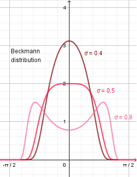
This was the Cook-Torrance specular reflection model. Nowadays a common model is GGX by Walter et al, for which people have done many good explanations about. It follows the same general form, but just has different distribution and geometry terms. Of course one can also mix different geometry, distribution and even the Fresnel approximation terms to get the result they are happy with.
Links
- A Reflectance Model for Computer Graphics (1982) - Robert L. Cook, Kenneth E. Torrance.
The original paper about the Cook-Torrance reflectance model. - Physically Based Rendering: From Theory To Implementation, Reflection Models / Microfacet Models (2018) - M. Pharr, W. Jakob, G. Humphreys.
Very thorough online book about PBR with explanations and derivations, including the Oren-Nayar and Cook-Torrance models. - How Is The NDF Really Defined? (2013) - Nathan Reed.
Blogpost about the distribution function and how it relates to surface area.
Image-Based Lighting
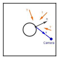
Remember that in the beginning we discarded the ambient light from consideration. This is why the objects in the Cook-Torrance example again look like they are in space. The light source we have is an ideal direction or ideal point, thus for a smooth surface reflection we also see an ideally small (depending on the smoothness) white dot. This is where image-based lighting comes in. We will try to estimate the directions of light that contribute to the reflectance towards our viewer direction. Then we can sample the scene or scene background at those directions and get the relevant ambient light.
Basically our problem is to find out where exactly should we sample and how much light from different directions contributes to the seen pixel color.
We will first look at the ideal diffuse case and then the specular one.
Diffuse
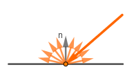
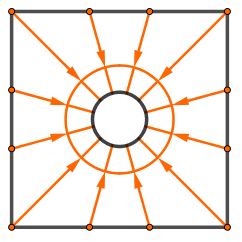
While we did saw the Oren-Nayar lighting model, in reality often still the ideal Lambertian diffuse reflectance is used. It is simple to work with and approximate as we will shortly see. The problem of incoming light for an ideal diffuse surface comes down to all the contributions from an hemisphere.
So in principle we could precalculate a cube map for (a static) scene by going through the different normals, sampling an hemisphere worth of colors, carefully averaging them together and saving the results. We would get a very low frequency map, which could be sampled in real time when we want to know the incoming ambient light.
Because the map itself would be low frequency, we can save storage space by creating and storing it in frequency domain instead. However, it is a very special frequency domain. Another reason for doing what we are about to do is that in that format there could also be somewhat dynamic light sources that can rotate or turn on/off in the scene. But we will not be going into that here.
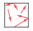
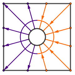
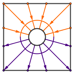
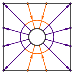
Instead of sampling the scene, we want to create and store a map of the light flow. You can think about light flow that if there is a relatively lighter and relatively darker areas in some particular direction, then there is flow of light there. We can record that flow of light as a single number (or 3 numbers in case of RGB). We just have to specify the particular directions. For example something like this:
 |
 |
 |
 |
 |
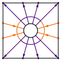 |
You can see that our first direction would be the average light in the entire scene. Then we could take the light moving from the right hemisphere to left. Then from top hemisphere to bottom. After that we can make the angles smaller and continue.
In 3D there are functions called spherical harmonics, which create such directions. There are infinitely many spherical harmonics functions and an algorithm for creating them. As the spherical harmonics functions are orthonormal functions, then they can serve as a basis for the light flow frequency space we want to create and store our scene in. If you are familiar with compression algorithms like JPEG, then you know that one way to save a lot of space is to discard the higher frequencies. In this method we are doing something similar. The more spherical harmonics we use, the closer to the actual result we get, but it turns out that it is already almost perfect if we just use something like 9 or 16 functions. We already established that the actual result would be quite low frequency anyway, even for a high frequency scene.
The spehrical harmonics come in sets called bands. Usually the band index is denoted $l$ and the index of the specific function inside the band is $m$. In each band there are $2 \cdot l - 1$ functions if $l$ starts from $1$. The index $m$ goes from $-l$ to $l$ and each function is usually denoted $Y_{l,m}$ or $Y_l^m$. Here are the first 9 spherical harmonics from the first 3 bands:
| $Y_0^{0} = c_1$ | ||||
| $Y_1^{-1} = c_2 \cdot \pmb{x}$ | $Y_1^{0} = c_2 \cdot \pmb{y}$ | $Y_1^{1} = c_2 \cdot \pmb{z}$ | ||
| $Y_2^{-2} = c_3 \cdot \pmb{x \cdot y}$ | $Y_2^{-1} = c_3 \cdot \pmb{y \cdot z}$ | $Y_2^{0} = c_4 \cdot (3 \cdot \pmb{z^2} - 1)$ | $Y_2^{1} = c_3 \cdot \pmb{x \cdot z}$ | $Y_2^{2} = c_5 \cdot \pmb{(x^2 - y^2)}$ |
Where the constants are: $c_1 = 0.282095$, $c_2 = 0.488603$, $c_3 = 1.092548$, $c_4 = 0.315392$ and $c_5 = 0.54627$.
You can see that each new band consists of higher polynomials on the input vector coordinates.
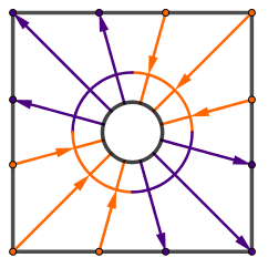
On the right there is an example how these functions describe the different directions for sampling the flow of light.
Now that we have the spherical harmonics functions, we want to use those as a basis for storing our scene lighting. The idea is that we go through as many vectors from an hemisphere as we can, and for each vector we:
- Sample the scene light (for example from the skybox) at that direction.
- For each used $Y$ (currently 9) get the weight of $Y$ for that direction ($Y(v)$).
- Multiply the sample and particular $Y(v)$ together.
- Accumulate the result with every vector for every $Y$ we use.
In the end we multiply all the accumulated results by $4 \cdot \pi$, because we are working on the surface of a sphere, and then divide by the number of different vectors we accumulated.
This gets us 9 numbers (or triplets), which represent the scene lighting in the spherical harmonics base. Let's call them scene coefficients. We can send these numbers to our diffuse shaders when rendering objects in that particular scene. To get back from those numbers to a particular color, we have to:
- Find the current surface normal in spherical harmonics space, by sending it to $Y(n)$ for each $Y$.
- Multiply the previously stored scene coefficients with the just found corresponding surface normal coefficients.
- Account for the dot product between the surface normal and incoming light vectors accumulated in scene coefficients by multiplying each coefficient by a specific factor $A_n$.
What happens in step 3. is that we are moving our Lambertian ideal diffuse BRDF into the spherical harmonics space and multiplying it with each coefficient to apply it. The coefficients of the $n \cdot \omega$ in the spherical harmonics space for all the harmonics in the first 3 bands are $A_0 = \pi$, $A_1 = 2.0943$, $A_2= 0.7853$. This step could also be done before on the CPU side.
Because of the low frequency of the map, this reconstruction of lighting could be done via Gouraud shading. Meaning that it can be done in a vertex shader and then interpolated across the fragments.
On the example to the right there is a diffuse object in the middle of an environment. You can change different environments, each environment has their own spherical harmonics coordinates already pre-calculated for use in this example. Notice that there actually are not any analytical light sources in the scene. All the illumination comes pre-calculated from the environment's cube map via spherical harmonics.
You can also turn off and on the different stored spherical harmonics coefficients on the example to see their contribution. They are called $L_l^m$, because they are the pre-computer coordinates of the scene lighting in the spherical harmonics space, not just the basis functions $Y_l^m$.
Something to consider in this algorithm is that if the lighting comes from an image, then we should know are the colors in linear or gamma space. If you want everything to look like it would if you open the image in your default image viewing software, then you need to gamma decode the colors after sampling them during the scene light flow map creation.
This technique of using spherical harmonics in computer graphics for a diffuse environment map was described by Ravi Ramamoorthi and Pat Hanrahan in their 2001 article. It has since been used in different game engines and algorithms.
Links
- An Efficient Representation for Irradiance Environment Maps (2001) – Ravi Ramamoorthi, Pat Hanrahan.
The article that brought spherical harmonics into use in computer graphics. - Spherical Harmonic Lighting: The Gritty Details (2003) – Robin Green.
Thorough explanation of spherical harmonics in computer graphics. Starts with the basics, but goes off the deep end. - Spherical Harmonics – Benoît Mayaux.
Practical overview of spherical harmonics in computer graphics.
Specular
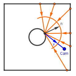
Let's observe how we would sample the environment via specular reflection in microfacets.
We need to notice here that the amount of the environment's contribution is not only dependent on the distribution, but also on the viewer angle. The sample at a grazing viewing angle contributes more than a sample at an angle near the surface normal. Even without the Fresnel term, which is obvious, we also had the normalization term depending on the viewer angle, because our functions work on half-angle vectors, not incoming light direction vectors. This is how the whole rendering equation looked like (without the emission term):
$$L_{out} = \int_\Omega L_{in}(\omega) \cdot (n \cdot \omega) \cdot {{F(h) \cdot D(h) \cdot G(\omega, v, h)} \over {4 \cdot (n \cdot v) \cdot (n \cdot \omega)}} ~ \mathrm{d} \omega $$
You can notice from the formula also the dependence on the viewer vector $v$. This means that differently from the diffuse case, here we have data points for every combination of normal, view vector and roughness values. This is too much to hold inside a single data structure. Thus we are going to separate it into approximated values for every normal and roughness combinations and correction values for every $(n \cdot v)$ and roughness combinations.
The algorithm that does this was popularized by Brian Karis from Epic Games in the 2003 article linked in the beginning of this entire topic and also described in the LearnOpenGL site. Before we get to it, remember that the ${4 \cdot (n \cdot v) \cdot (n \cdot \omega)}$ factor was for normalizing the distribution term $D$ to be over half-angles. Let's move that part inside the $D$ function itself, so the formula will be shorter to write. The main idea of the algorithm is to factor this integral into 2 parts like this (with the just mentioned normalization factor moved inside $D$):
| $$L_{out}~=~$$ | $${\displaystyle\int_\Omega L_{in}(\omega) \cdot (n \cdot \omega) \cdot F(h) \cdot D(h) \cdot G(\omega, v, h) ~ \mathrm{d} \omega} \over {\displaystyle\int_\Omega F(h) \cdot D(h) \cdot G(\omega, v, h) ~ \mathrm{d} \omega}$$ | $$\cdot$$ | $$\int_\Omega F(h) \cdot D(h) \cdot G(\omega, v, h) ~ \mathrm{d} \omega$$ |
| We are going to approximate this part... | ...and use this part to correct for the approximation. |
The first thing we'll do is replace all the integrals with sums. This means that we will be estimating them via some chosen Monte-Carlo method. Importance sampling is the recommended approach. It means that we will be using our distribution to get sample vectors from. If our distribution is Beckmann as it is in the Cook-Torrance model, then we take some sample vectors $l ⬿ Beckmann$. The actual distribution is also dependent on the roughness value, so we will have to do this for every roughness. For now, we just fix one and continue.
When moving from those integrals to sums, we will lose the distribution term (as we are already sampling $l$ vectors from it). Important to note is that, again, our distribution was over half-angles, but we will create sample (for example $l$) vectors uniformly over the hemisphere. It turns out that to use the Beckmann distribution of half-angle vectors and Monte-Carlo over $l$ vectors according to the given distribution, we have to multiply with a factor ${4 \cdot v \cdot h} \over {D \cdot n \cdot h}$. When we do this multiplication, we get (now we bring the normalization factor out of $D$ again):
$${\color{darkgray}{(n \cdot l)} \cdot {F(h) \cdot \color{darkgray}{D(h)} \cdot G(l, v, h)} \over {4 \cdot (n \cdot v) \cdot \color{darkgray}{(n \cdot l)}}} \cdot {{\color{darkgray}{4} \cdot v \cdot h} \over {\color{darkgray}{D} \cdot n \cdot h}} = $$
$$= {{F(h) \cdot G(l, v, h)} \over {(n \cdot v)}} \cdot {{v \cdot h} \over {n \cdot h}} = F(h) \cdot G(l, v, h) \cdot {{v \cdot h} \over {(n \cdot v) \cdot (n \cdot h)}}$$
So our formulae will now look like this:
| $$L_{out}~=~$$ | $${{1 \over N} \cdot \displaystyle\sum_l L_{in}(l) \cdot F(h) \cdot G(l, v, h) \cdot {v \cdot h \over (n \cdot v) \cdot (n \cdot h) }} \over {{1 \over N} \cdot \displaystyle\sum_l F(h) \cdot G(l, v, h) \cdot {v \cdot h \over (n \cdot v) \cdot (n \cdot h)}}$$ | $$\cdot$$ | $${1 \over N} \cdot \displaystyle\sum_l F(h) \cdot G(l, v, h) \cdot {v \cdot h \over (n \cdot v) \cdot (n \cdot h)}$$ |
Are you not happy we got rid of the neat integrals in favor of sums? No worries, we will simplify these sums a bit. Let's start with the left part of the whole product. The term we are going to approximate. The approximation Karis described was that we assume the viewer is always looking perpendicular to the surface. Meaning:
$$v = n = r$$
This has some implications on the actual reflections we get, but it allows to create an irradiance map only based on the normal direction. Instead of both normal and view vectors.
With this approximation we can really simplify the left term. First $n \cdot v = 1$, because $n = v$, so we can remove it:
$${{1 \over N} \cdot \displaystyle\sum_l L_{in}(l) \cdot F(h) \cdot G(l, v, h) \cdot {v \cdot h \over \color{darkgray}{(n \cdot v)} \cdot (n \cdot h) } \over {1 \over N} \cdot \displaystyle\sum_l F(h) \cdot G(l, v, h) \cdot {v \cdot h \over \color{darkgray}{(n \cdot v)} \cdot (n \cdot h)}} = {{1 \over N} \cdot \displaystyle\sum_l L_{in}(l) \cdot F(h) \cdot G(l, v, h) \cdot {v \cdot h \over n \cdot h } \over {1 \over N} \cdot \displaystyle\sum_l F(h) \cdot G(l, v, h) \cdot {v \cdot h \over n \cdot h}}$$
Secondly, $v \cdot h = n \cdot h$, again because $v = n$. This means it cancels out in the fraction, leaving $1$, which we can remove:
$${{1 \over N} \cdot \displaystyle\sum_l L_{in}(l) \cdot F(h) \cdot G(l, v, h) \cdot \color{darkgray}{v \cdot h \over n \cdot h } \over {1 \over N} \cdot \displaystyle\sum_l F(h) \cdot G(l, v, h) \cdot \color{darkgray}{v \cdot h \over n \cdot h}} = {{1 \over N} \cdot \displaystyle\sum_l L_{in}(l) \cdot F(h) \cdot G(l, v, h) \over {1 \over N} \cdot \displaystyle\sum_l F(h) \cdot G(l, v, h)}$$
Thirdly we are going to set the geometry term $G$ to $1$. If we are looking straight down, there should not be masking with V-cavities in our model. The incoming light could be shadowed, but only at large angles, which have a low probability because of our distribution and if we assume not too big roughness.
$${{1 \over N} \cdot \displaystyle\sum_l L_{in}(l) \cdot F(h) \cdot \color{darkgray}{G(l, v, h)} \over {1 \over N} \cdot \displaystyle\sum_l F(h) \cdot \color{darkgray}{G(l, v, h)}} = {{1 \over N} \cdot \displaystyle\sum_l L_{in}(l) \cdot F(h) \over {1 \over N} \cdot \displaystyle\sum_l F(h)}$$
For the Fresnel term, let's look at the Schlick's approximation: $F(n, v) = R_0 + (1 - R_0) \cdot (1 - n \cdot v)^5$. Because $n \cdot v = 1$, we get that the Fresnel approximation is constant $F(n, v) = R_0$. We can thus bring this outside of the sum, where it factors out:
$${{1 \over N} \cdot \displaystyle\sum_l L_{in}(l) \cdot \color{orange}{F(h)} \over {1 \over N} \cdot \displaystyle\sum_l \color{orange}{F(h)}} = {{1 \over N} \cdot \displaystyle\sum_l L_{in}(l) \cdot \color{red}{R_0} \over {1 \over N} \cdot \displaystyle\sum_l \color{red}{R_0}} = {\color{red}{R_0} \cdot {1 \over N} \cdot \displaystyle\sum_l L_{in}(l) \over \color{red}{R_0} \cdot {1 \over N} \cdot \displaystyle\sum_l 1} = {{1 \over N} \cdot \displaystyle\sum_l L_{in}(l) \over {1 \over N} \cdot \displaystyle\sum_l 1}$$
If we check out what is going on the denominator, we get that summation $N$ times the number $1$, will get us $N$, which is then factored out after the summing. This leaves us with just a single sum for our approximation:
$${{1 \over N} \cdot \displaystyle\sum_l L_{in}(l) \over {1 \over N} \cdot \color{orange}{\displaystyle\sum_l 1}} = {{1 \over N} \cdot \displaystyle\sum_l L_{in}(l) \over {1 \over N} \cdot \color{orange}{N}} = {1 \over N} \cdot \displaystyle\sum_l L_{in}(l)$$
This sum says that for the first approximated part of our result, we need to create some sample vectors from our distribution and then sample our environment map with them. We sum the samples and then average over the total number of samples we took. Nice, that is easy to do and we can store the result in a cube map.
Now, for the right term. The visual effects that were approximated by the left side were the geometry and the Fresnel effect. So with the right part we would like to somehow re-add the geometry term and correct (with scale and translation/bias) the Fresnel term. In addition to that we also have the distribution conversion factor for importance sampling to calculate. Let's call the latter $m$, because it unfortunately will not cancel out this time.
$${1 \over N} \cdot \displaystyle\sum_l F(h) \cdot G(l, v, h) \cdot \color{red}{v \cdot h \over (n \cdot v) \cdot (n \cdot h)} = {1 \over N} \cdot \displaystyle\sum_l F(h) \cdot G(l, v, h) \cdot \color{red}{m}$$
When we look at the Fresnel effect approximation, we can see that the $n \cdot v$ term (which we approximated before) contributes both multiplicatively and additively. This is where we will get our scale and bias terms:
$$F(n, v) = R_0 + (1 - R_0) \cdot (1 - n \cdot v)^5 = R_0 + (1 - n \cdot v)^5 - R_0 \cdot (1 - n \cdot v)^5 = R_0 \cdot (1 - (1 - n \cdot v)^5) + (1 - n \cdot v)^5$$
Previously with the left term we saw that $F$ gave us just $R_0$ (which cancelled out). So our approximation of the Fresnel effect was $R_0$. Now we can see that to get the actual result, we need to multiply $R_0$ with $(1 - (1 - n \cdot v)^5) $ and add to it $(1 - n \cdot v)^5$. We are going to use this to split the sum into two, because we are interested in both of these terms individually:
$${1 \over N} \cdot \displaystyle\sum_l \color{orange}{F(h)} \cdot G(l, v, h) \cdot m = {1 \over N} \cdot \displaystyle\sum_l (\color{brown}{R_0 \cdot (1 - (1 - n \cdot v)^5)} + \color{olive}{(1 - n \cdot v)^5}) \cdot G(l, v, h) \cdot m = $$
| $$=$$ | $$ {1 \over N} \cdot \displaystyle\sum_l (\color{brown}{R_0 \cdot (1 - (1 - n \cdot v)^5)}) \cdot G(l, v, h) \cdot m$$ | $$+$$ | $${1 \over N} \cdot \displaystyle\sum_l \color{olive}{(1 - n \cdot v)^5} \cdot G(l, v, h) \cdot m$$ |
| Scale | Bias |
We are also going to remove the $R_0$ from the scale term. The actual value for $R_0$ is calculated later, when we are rendering our scene. We just need to know the scale factor to multiply it with.
Nice. This allows us to correct for the error we made in the approximation. We get different correction values for different view vectors $v$ (or more specifically, for different values of $v \cdot n$). We can store those in a line texture and use the red channel for the scale term and the green channel for the bias term.
One thing that is currently missing is roughness. For different roughness values we have different distributions of sample vectors. So we need to calculate both the left and right terms for different roughness values. For the right side we can just extend our line texture into 2D, the second axis being the roughness value. For the left hand irradiance cubemap it is more tricky. The solution described by Karis saves the different results into the mipmaps of the cubemap.
Putting this together we should be able to pre-calculate values like these via the described approach:
| Formulae: | Approximated scene irrandiance. | Correction for the approximation. | |
| $$L_{out}~=~$$ | $${\displaystyle\int_\Omega L_{in}(\omega) \cdot (n \cdot \omega) \cdot F(h) \cdot D(h) \cdot G(\omega, v, h) ~ \mathrm{d} \omega} \over {\displaystyle\int_\Omega F(h) \cdot D(h) \cdot G(\omega, v, h) ~ \mathrm{d} \omega}$$ | $$\cdot$$ | $$\int_\Omega F(h) \cdot D(h) \cdot G(\omega, v, h) ~ \mathrm{d} \omega$$ |
| Monte-Carlo importantce sampling: | |||
| $$L_{out}~=~$$ | $${1 \over N} \cdot \displaystyle\sum_l L_{in}(l)$$ | $$\cdot$$ | $$\left({1 \over N} \cdot \displaystyle\sum_l (\color{brown}{(1 - (1 - n \cdot v)^5)}) \cdot G(l, v, h) \cdot m + \\ {1 \over N} \cdot \displaystyle\sum_l \color{olive}{(1 - n \cdot v)^5} \cdot G(l, v, h) \cdot m \right)$$ |
| Results: | 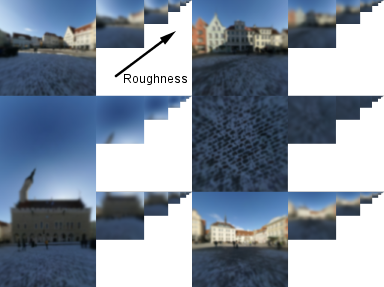 |
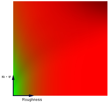 |
|
| Cubemap, with mipmaps for different roughness levels. | Correction map. Corrects based on the view vector. | ||
Note that the cubemap with mipmaps here is rescaled and modified for display purposes. One file format to store this in would be DDS. There is a plugin for Photoshop named NVIDIA Texture Tools, that allows you to open and change DDS files. It supports cubemaps and cubemap mipmaps. Another tool to just view DDS files would be ddsview from amnoid.de.
Very good. Now the last step is to use this data when rendering. We started the entire process from $L_{out}$, so the final specular color will be pretty much just a combination of the samples from these pre-created textures. Only thing is that we need to also plug in an actual value for $R_0$, which we calculate for different materials. Because our correction map also includes the geometry term, we need to calculate the actual Fresnel response in real time as well. After that we can just blend the diffuse and specular values together just like before, but for the specular we get:
| $\mathrm{IrradianceCube}(r, roughness)$ | $ \cdot $ | $( R_0 \cdot \mathrm{CorrectionTex}(n \cdot v, roughness).red $ | $ +$ | $ \mathrm{CorrectionTex}(n \cdot v, roughness).green $ | $ ) $ |
| Incoming light approximation | Geometry term and Fresnel scale correction | Fresnel bias correction |
The vector $r$ there is the reflection vector. There are different code examples in both the linked article by Karis and the LearnOpenGL site if you are more interested in implementation. Although depending on the source, some details may be conveyed differently.
On the right there is the example using this algorithm. Naturally the spherical harmonics from the previous section have also been integrated here.
I have capped the standard deviation parameter $\sigma$ to 1 and called it "r" for roughness. This parameter can be rescaled for convenience depending on the use case.
You can also notice that at some higher roughness levels the reflections become a bit smudgy. This is especially noticeable in the ColorBox scene. It is because the mipmaps get so low level that the small amount of pixels define a too hard gradient.
One more problem with this mipmap approach is that the sharpest levels of mipmaps would get some aliasing. Initially when the surface was almost completely smooth, I sampled the mipmap level 0, which corresponded to $\sigma = 0$ roughness. But because there were not any regular mipmaps and the object was small on the viewport, there was horrible sampling alias. One solution for this is to use the environment map (full scale cubemap with regular mipmaps) for sampling in case of smooth surface. Then quickly interpolate those results to the generated irradiance map mipmaps when roughness increases. This seems to work pretty well.
Great! Now you should have good tools for understanding physically-based rendering and go read (and understand) the different linked sources on the topics. Especially what was done in UE and Frostbite engines and described in the articles linked in the first section.
Link
- Specular IBL – LearnOpenGL.
Very good practical overview of the described technique. - Sampling microfacet BRDF (2015) – Jiayin Cao.
Derivations of generation functions for different distributions (Beckmann, GGX, Blinn) - Alternative Take on the Split Sum Approximation for Cubemap Pre-filtering (2019) – Evgenii Golubev.
Blogpost that helps to understand how the rendering equation is approximated in this technique.